Estimated Temporal Variation of Losses Due to a Recurrence of the 1933 Long Beach Earthquake

Abstract

The temporal variation of damage and loss estimates are presented in decadal increments since 1950 for an earthquake on the Newport-Inglewood Fault (NIF) equivalent to the M_w 6.4 1933 Long Beach earthquake. Deterministic damage and loss calculations were performed utilizing Hazus-MH software and updated structural inventories. We estimate that building stock loss density (total losses within each census tract divided by tract area) due to the recurrence of this event in 1950 would have been about $84 million, increasing to $300 million in 2006 (2002 replacement costs). With the phenomenal growth in new construction in Long Beach over the past 50 years, the results indicate that the proportion of wood and unreinforced masonry (URM) buildings predicted to suffer at least moderate damage has stabilized. Given the many seismic sources in this region which also pose significant threats, we demonstrate that modeling tools such as Hazus-MH can provide meaningful estimates of future losses from earthquakes.

Introduction

The M_w 6.4 1933 Long Beach, California earthquake was one of the most devastating in the history of the United States, both in terms of human suffering and economic impact (Benioff 1938, Hauksson 1987, Hauksson and Gross 1991, Grant et. al. 1997, Housner 2002). Today, dense residential and commercial structural inventory have been rebuilt right on top of the fault that generated this event. In the 1933 event, approximately 120 people lost their lives while thousands more were injured and displaced. Most of the structural damage occurred in dense suburbs and commercial areas; saturated alluvium and substandard buildings increased the losses. An estimated $40–$50 million (in 1933 dollars) in total property losses occurred in the cities of Long Beach and Compton, where observed intensities reached IX on the 1931 modified Mercalli scale (Martel 1965, Campbell 1976, SCEC 2009). Similar, more recent events in California, have had devastating effects on local populations, such as the M_w 6.7 1994 Northridge earthquake. Fatalities due to this event totaled 33, 24 of whom were killed as a result of damage to wood-framed buildings; 16 of those were in a single structure with tuck-under parking (Northridge Meadows apartment complex). Injuries were estimated at 9,000, and the American Red Cross was required to provide shelter for up to 17,500 people at any given time immediately following the event. Building-related and overall economic losses as a result of that disaster totaled approximately $20 and $44 billion, respectively (Comerio et. al. 1996, EQE International, Inc. 1997, Eguchi et. al. 1998). In addition, damage to wood-framed structures caused more than $20 billion in property loss, exceeding the financial loss from any other single type of building construction from the quake.

The 1933 Long Beach earthquake occurred on the Newport-Inglewood fault zone (NIFZ), which forms the western margin of the Los Angeles Basin in Southern California (Figure 1). Although the repeat time of the Long Beach earthquake is anticipated to be on the order of several thousand years, the severity of this event showed that this fault zone should be considered active and capable of generating damaging events (Ziony et. al. 1985, California Division of Mines and Geology 1988, Dolan et. al. 1995). A recurrence of this or a similar earthquake presents a very real threat to the population of Long Beach as well as to the surrounding cities within the Los Angeles area, regardless of exactly where an event might initiate along the segment of the fault which previously ruptured.

Figure 1.

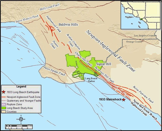
Map of Los Angeles area showing our study area relative to the NIFZ (Bryant 2005) and the 1933 fault rupture zone (Hauksson 1987) along the north branch of the NIF. The upper right inset depicts study area relative to surrounding region.

The potential impact of such an event on Los Angeles is currently a subject of great interest (e.g., ASCE 2003, EERI 2006, City of Los Angeles 2009). With regard to previous estimates of risk to this area, the Federal Emergency Management Agency (FEMA) performed a study (FEMA 2008b) to estimate seismic risk in all regions of the United States using Hazus-MH MR2 software to determine the annualized earthquake loss (AEL), or the long-term value of earthquake losses to the general building stock in any single year in a specified geographic area (i.e., state, county), and the annualized earthquake loss ratio (AELR), which is the annualized loss (AEL) as a fraction of the building inventory replacement (2002) value. The AELR is a loss-to-value ratio expressed in terms of dollars per million dollars of building inventory exposure. The results of this analysis anticipated the AEL and the AELR for the Los Angeles–Long Beach–Santa Ana metropolitan area to be $1.31 billion and $1.75 billion, respectively, among the highest in the nation. In AEL and AELR, this regions ranks first and fifth in the nation, with respect to potential losses. The measures reflect the distribution of relative earthquake risk across the nation, and thus represent a much broader measure of risk than this study.

The current study sought to forecast the direct economic loss to the current structural inventory in the Long Beach vicinity as accurately as possible, should an event similar to the 1933 Long Beach earthquake occur in 2010. Variations of the historical earthquake magnitude are also considered in order to quantify and compare losses. Although effects of directivity are another important factor to consider when estimating losses, this will be considered in later studies. This study utilized Hazus-MH MR1 (Maintenance Release 1) standardized methodology augmented with an updated structural inventory for the city of Long Beach and Hazus-MH MR3 (Maintenance Release 3) to conduct risk analyses in ten-year increments from 1950 to 2000, and for 2006. Hazus-MH software was originally developed by FEMA and the National Institute of Building Sciences (NIBS). Hazus-MH can be utilized to estimate potential losses from earthquakes, hurricane winds, and floods anywhere in the United States. The Hazus-MH methodology is integrated with the Environmental Systems Research Institute's (ESRI) proprietary geographic information systems (GIS) software, ArcGIS, so it is particularly suited to mapping and visualizing natural hazards as well as damage and economic loss estimates for buildings and infrastructure and the respective impacts on affected populations.

The Long Beach Earthquake

The Long Beach earthquake struck at 5:54 p.m. on 10 March 1933. Both the focal mechanism of the main shock and the aftershock distribution indicate that the event occurred on the northern branch of the Newport-Inglewood Fault (NIF), 8 km to 20 km beneath southern Huntington Beach (Figure 1) (Benioff 1938, Hauksson and Gross 1991, Grant et. al. 1997). The NIF is but one segment within the NIFZ, which strikes northwest subparallel to the San Andreas Fault, and extends from the Santa Monica Fault in the north to Newport Beach in the south, then seaward more than 250 km south into Baja California (Ziony and Yerkes 1985, Hauksson 1987). This fault zone exhibits a right-lateral strike-slip component of motion (Yerkes et. al. 1965, Barrows 1974).

The 1933 fault rupture extended for 13 km to 16 km from the city boundary of Huntington Beach and Newport Beach toward the northwest along the NIF. An estimated 85 cm to 120 cm of slip occurred at depth along the rupture surface due to the main shock (Hauksson and Gross 1991), while the long-term slip rate of the NIF is estimated to be between 0.1–1.0 mm/yr (Ziony and Yerkes 1985). A geotechnical investigation by Grant et. al. (1997) revealed that the northern branch of the NIFZ in Huntington Beach has generated up to five recognizable surface ruptures indicative of similar or greater magnitude earthquakes within the past 12,000 years. In addition, various investigations have indicated that unconsolidated soil conditions contributed to much of the observed damage and subsequent casualties (Martel 1965, Campbell 1976). For example, Campbell (1976) scrutinized the relative amounts of damage sustained by buildings on older versus recent alluvium and found that at any given distance from the NIF, the amount of observed damage was greater on recent as opposed to older alluvium.

Following the 1933 event, approximately 40 school buildings collapsed and 120 were damaged in Long Beach and surrounding areas, which led to much greater public awareness of building safety (Olsen 2003). The quake occurred at about 5:54 p.m. Pacific Standard Time, but if it had occurred during school hours the fatalities related to the destruction of the schools would have been much higher. Many of the schools were brick buildings with unreinforced masonry walls. Engineered and reinforced concrete buildings suffered little or no structural damage in the earthquake. This study focuses on the city of Long Beach, since the city experienced such considerable structural damage as well as fatalities due to the earthquake. An estimated two-thirds of the deaths attributed to the event were caused by falling debris as people attempted to escape buildings. The focus on a single city within the Los Angeles area is also the result of practical limitations of purchasing and preparing the updated detailed structural inventories and the processing time required for computing losses for multiple earthquake scenarios.

Structural Inventories: 1950–2006

The default building stock and associated exposure (replacement value) tables in Hazus-MH MR1 were replaced with accurate structural inventory information to generate multiple historical estimates of potential earthquake losses in the Long Beach area. Manual processing of structural inventory information such as assessor data is required prior to performing a “high priority” building inventory update in the Hazus-MH MR1 environment (ImageCat and ABS Consulting 2006a, Swift et. al. 2009). The ImageCat and ABS Consulting (2006a, 2006b) data standardization guidelines for loss estimates using the building inventory replacement tool (BIRT) in Hazus-MH MR1 were fully utilized to perform the structural inventory updates, as detailed herein. Current structural inventory data for a total of 35 zip codes in the city of Long Beach were purchased directly from the Los Angeles County Office of the Assessor (Los Angeles County 2010a). The raw data were inspected for completeness and carefully geocoded to Long Beach parcel boundary information obtained from the Los Angeles County Office of the Assessor. At each step in the following procedure the data were manually reviewed using a combination of visual mapping and manual validation where approximately 2% of the building/parcel data were randomly chosen and spot checked against the current Office of the Assessor property search Web page (Los Angeles County 2010b). The 276 different Office of the Assessor property use classifications within the raw dataset were then translated into 33 Hazus-MH MR1 occupancy classes and associated standard industrial classification (SIC) codes (OSHA 2009, FEMA 2008b). Additional data preparation steps were required such as the assignment of Hazus-MH MR1 occupancy classes to 2,765 apartment buildings possessing different numbers of apartment units. In this step, structures located in 4,885 parcels with assessor use codes representing five or more apartment units (05xx) were sorted into the appropriate Hazus-MH MR1 occupancy class based on the number of units.

Building counts, building square footage, occupancy, year of construction, value, and location were aggregated for each of seven datasets based on Hazus-MH MR1 occupancy classes, one dataset for each decade considered. Subsequently, six additional inventories were defined according to year of construction by filtering the 2006 dataset according to structures built by 1950, 1960, 1970, 1980, 1990, and 2000 into individual datasets. Each dataset included information on buildings constructed up to and including the specified year. For each decade considered, each dataset contained 117 census tracts comprised of over 120,000 parcels. Each of the seven datasets were then stored in Microsoft Access database templates designed to be imported into Hazus-MH MR1 for the next step in the analysis (ImageCat and ABS Consulting 2006b, 2006c).

The next step in data preparation involved uploading the historical structural inventories as seven different Hazus-MH MR1 “study regions” using the ImageCat and ABS Consulting (2006b) BIRT prior to running the earthquake loss estimates on each dataset. The default square footage and building count information were replaced within each Hazus-MH MR1 study area (decade) with the aforementioned assessor data. The Hazus-MH MR1 mapping schemas for each decade, which define the overall percent distribution of building square footage according to occupancy across basic structural types, such as wood, masonry, concrete, or steel, were also updated accordingly. This resulted in completely updated building counts, square footage values, and related exposure tables within each of the seven study region datasets to which BIRT was applied. Compared to the computed year 2000 results, the default Hazus-MH MR1 (dated 2002) values overestimated the building count by 14% and underestimated square footage by 7%. Figure 2 shows that the total building count has roughly doubled, while the square footage has more than tripled since 1950. Figure 3 shows the temporal variation in the distribution of buildings by occupancy type, illustrating the growth of residential versus nonresidential building stock in the study area over the last 50 years.

Figure 2.

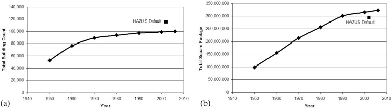
Updated structural inventory: a) total building count and b) square footage for each decade (diamonds) with respect to the default Hazus-MH MR1 2002 values (squares).

Figure 3.

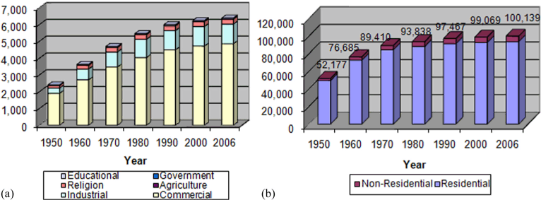
(a) Total building counts as a function of age and general occupancy types and (b) breakdown of nonresidential building types. Total counts for all building types are provided at the top of each column in a)

Lastly, each of the seven study region datasets were exported from Hazus-MH MR1 and imported into Hazus-MH MR3 to perform the loss estimates using the most up-to-date building damage and loss computations available (FEMA 2007). Each imported decade dataset was checked against the original study regions generated using BIRT by manually comparing both inventory data and mapping schemas for consistency prior to conducting the analysis.

This approach meant that exposure values in terms of both amount and basic construction type have been modified to reflect growth over time. Although buildings of different ages incorporated different structural vulnerabilities, these vulnerabilities were not explicitly modified by the update to the general mapping scheme. In order to adjust for changes in specific structural vulnerability over time, additional modifications to the mapping scheme or custom building attribute mapping schemes would need to be devised and implemented in Hazus (i.e., Kircher et. al. 2006). Specific structural information such as building height and seismic design level were not available for this study.

The building codes introduced since the 1970s have had a significant impact on advancing earthquake safety. In general, buildings designed and constructed according to the newer codes are anticipated to perform better during earthquakes. Structures built prior to 1980 are less likely to meet current code requirements, and thus are more likely to suffer damage. Figure 4 depicts the spatial distributions of older versus newer buildings as well as the growth in terms of construction over time in the study area. Replacing the Hazus-MH MR1 default structural inventory with current data from the Office of the Assessor for a particular study area takes building vintage into account by updating the general, rather than specific, building mapping schemes, and by improving density information by census tract. Specific mapping schemes that reflect the structural vulnerabilities such as unreinforced versus reinforced masonry and nonductile versus ductile concrete frame were not taken into account. This means that the updated Hazus-MH MR1 general building mapping schemes reflect basic construction materials only, and do not incorporate updated information on specific structural systems or building height. However, no changes were made to specific mapping schemes within Hazus-MH MR1; thus building types not presently accommodated in Hazus were not taken into account, such as newly retrofitted structures (Kircher et. al. 2006).

Figure 4.

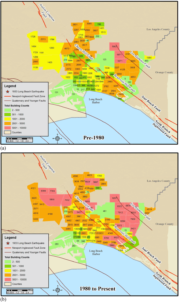
Maps of (a) older relative to (b) newer construction based on the building counts in the assessor's inventory data. Values refer to total building counts per census tract for pre-1980 versus post-1980 categories.

Analysis

The M_w 6.4 1933 Long Beach earthquake was chosen as the primary scenario event for this analysis. This earthquake is considered to be within the “geological reasonable scenarios” as defined by Dolan et. al. (1995). In addition, variations of this scenario were implemented for moment magnitudes 6.0, 6.4, 6.8, and 7.2 coupled with the same source parameters (Hauksson and Gross 1991) and combination attenuation function listed in Table 1. Hauksson and Gross (1991) source parameters utilized for the 1933 earthquake include a fault depth of 13 km, a focal mechanism strike of 315°, a dip of 80° to the northeast, and a rupture length of 15 km. The Hazus-MH MR3 methodology computes the fault rupture length based on the relationship of Wells and Coppersmith (1994) and assumes that the fault rupture is of equal length on each side of the epicenter (FEMA 2008a, Chapter 4). The ground motions were calculated using median predictions of the western United States (WUS) extensional shallow crustal attenuation functions. The WUS attenuation function weights each relationship in Table 1 equally (averages the median predictions), based on the methodology used by the United States Geological Survey (USGS) in 2002 to update the National Seismic Hazard Maps for California coasts (Frankel et. al. 2002, FEMA 2004, ASCE 2005).

Table 1

Combination attenuation relationships for extensional WUS shallow crustal event (from FEMA 2008a, Table 45)

Attenuation Functions
Abrahamson and Silva (1997)
Sadigh, Chang, Egan Makdisi, and Young (1997)
Boore, Joyner, and Fumal (1997)
Spudich, Joyner, Lindh, Boore, Margaris, and Fletcher (1999)
Campbell and Bozorgnia (2003)

Our intent was to focus on comparing damage estimates and losses due to credible events of different sizes that the current literature suggests might occur along the NIF. Field et. al. (2005) conducted a similar study using scenarios with different magnitudes combined with multiple accepted and commonly used attenuation functions in order to examine the effects of different models on resultant losses. This study utilizes the same earthquake parameters and attenuation function for all scenarios to examine the temporal variation of losses, rather than the influence of different ground motion models on outcomes.

In order to perform damage and loss estimates, Hazus-MH MR3 requires median shaking level maps for spectral acceleration (SA) at 0.3- and 1.0-second periods, peak ground velocity (PGV), and peak ground acceleration (PGA). Deterministic seismic ground motions for our specified scenario earthquakes were generated using Hazus-MH MR3 (FEMA 2007). A total of 28 sets of earthquake shakemaps (four magnitudes or scenarios, across seven decades) were generated. Several examples of the Long Beach shakemaps are provided in Figure 5. The maps generated for PGV, 0.3- and 1.0-second SA with respect to each magnitude are qualitatively similar to those in Figure 5, and thus are not displayed. It is apparent that, as would be expected, shaking increases with increasing magnitude and proximity to the source.

Figure 5.

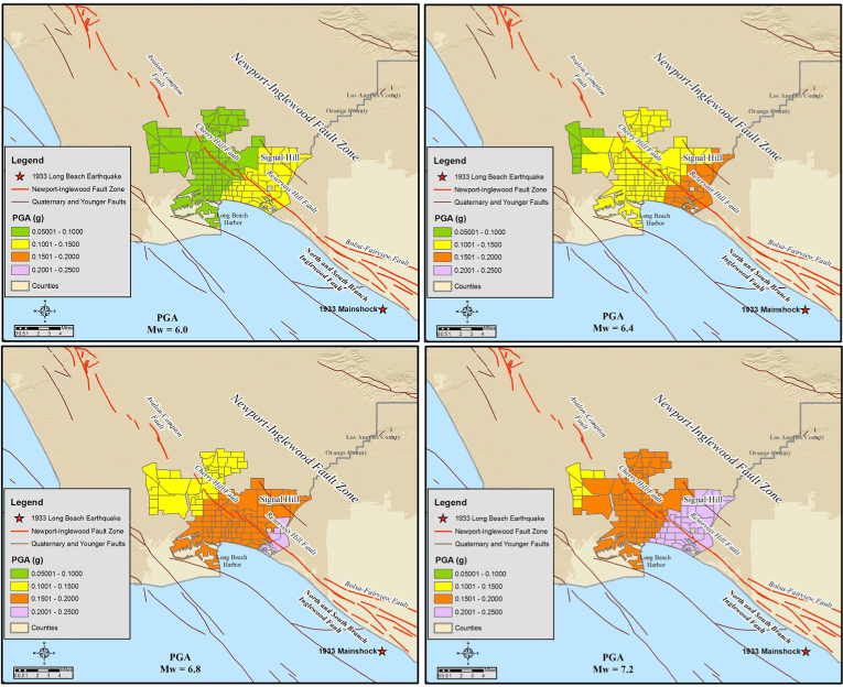
PGA maps as a function of the magnitude (M_w) 6.0, 6.4, 6.8, and 7.2 (top to bottom) Long Beach earthquake scenarios considered in this study. The coordinate bounds of the map are approximately 33.5° to 34.2° latitude and −118.6° to −117.8° longitude, whereas the study area boundary lies roughly within 33.7° to 33.8° latitude and −118.3° to −118.1° longitude.

Loss estimates were generated using Hazus-MH MR3 by applying the shakemaps to the updated assessor's structural inventories integrated into each study region dataset (decade). Damage predictions for ground shaking are utilized in the methodology to estimate monetary losses due to building damage (i.e., cost of repairing or replacing damaged buildings and their contents); in this study business inventory and building content values were not otherwise adjusted. Table 2 summarizes the building exposure for each temporal increment analyzed. In 1950, there were approximately 52,000 structures in the study area, whose value today would be $10 billion (excluding building contents and inventory related to business activities) (Figure 2). As of 2006, the number has nearly doubled to an estimated 100,000 buildings, with the total building replacement value exceeding $31 billion, the latter is a reflection, in part, of the tripling of square footage. Total populations and number of households normalized to Census 2000 data are also provided in Table 2 (Ethington et. al. 2000, Tatalovich and Wilson 2007). The Hazus-MH MR3 default Census 2000 population and household values of 530,819 and 182,228, respectively, were utilized in all 28 analyses in this study. No modifications were made to the default population data within Hazus-MH MR1 or MR3 because the fatality and other socioeconomic losses (i.e., wages) which are calculated for inventory data and various tabulated economic parameters for the earthquake scenarios are not addressed in this paper.

Table 2

Total number of buildings, square footage, and exposure for the 117 census tracts within the Long Beach study area

			Building Exposure (2002 $ replacement cost x 1,000)
Year	Total Building Count	Total Square Footage	Residential	Nonresidential	Total	Population¹⁾	Households¹⁾
1950	52,163	99,135,776	7,971,812	1,645,017	9,616,829	300,433	110,495
1960	76,671	156,137,250	11,947,110	3,127,732	15,074,842	378,831	147,765
1970	89,396	213,366,985	15,815,336	5,017,230	20,832,566	401,559	166,220
1980	93,824	256,253,247	17,389,804	7,381,122	24,770,926	407,642	176,635
1990	97,453	300,817,350	19,490,173	9,782,791	29,272,964	475,877	189,454
2000	99,055	314,504,698	19,958,201	10,533,948	30,492,149	537,147	194,277
2006	100,125	322,780,729	20,380,405	10,839,598	31,220,003	—	—

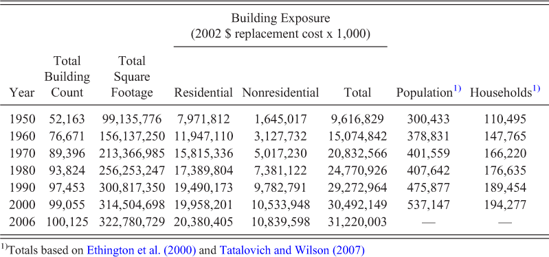
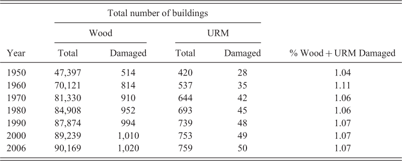
Totals based on Ethington et al. (2000) and Tatalovich and Wilson (2007)

For the M_w 6.4 scenario shown in Figure 5, the distribution of total economic exposure (i.e., replacement value as of 2002) with regard to building stock is illustrated in Figure 6 for 1950, 1980, and 2006. Exposure density is calculated by dividing the total building value within each census tract by the tract area (km²). Exposure density maps generated for this earthquake for each decade are incremental between these three decades in terms of spatial distribution of increasing exposure, so are not presented. From 1950 to 2006, overall building exposure in the study area increased three-fold. It is important to note that the Port of Long Beach and Long Beach Airport are not included in the exposure values, since they are integrated within the transportation systems in Hazus-MH MR1 and MR3, which are not considered in this study. In general, Figure 6 indicates that exposure has increased over time, most notably in census tracts in southern Long Beach where there has been substantial growth in residential, commercial, and industrial building stock over the last 60 years. Table 3 provides a summary of the anticipated damage to all design levels of the most common (wood) and most vulnerable (URM) building types analyzed in this study, based on the M_w 6.4 scenario. The proportion of wood and URM buildings predicted to suffer at least moderate damage with respect to total building count for each decade is provided. In Hazus-MH MR3, moderate damage to URM buildings is defined as diagonal cracks in wall surfaces, visible separation of walls from diaphragms, significant cracking of parapets, or fallen parapet or wall masonry (FEMA 2008a). Moderate damage to light-frame (W1) wooden buildings is defined as large plaster or gypsum-board cracks at the corners of door and window openings, small diagonal cracks across shear wall panels exhibited by small cracks in stucco and gypsum wall panels, large cracks in brick chimneys, or toppling of tall masonry chimneys; for commercial and industrial (W2) wooden buildings, moderate damage is defined as larger cracks at the corners of door and window openings, small diagonal cracks across shear wall panels, minor slack in diagonal rod bracing requiring re-tightening, minor lateral set at store fronts and other large openings, or small cracks or wood splitting at bolted connections. The leveling off of expected damage indicated in the later decades (Table 3) is most likely related to a decrease in both the rate of construction and in the percentage of URM structures with respect to overall building inventory in the study area.

Figure 6.

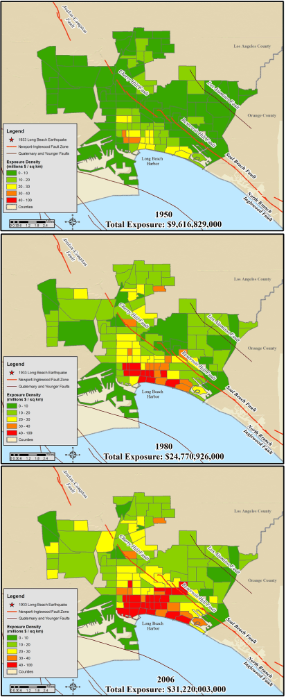
Spatial distribution of total building exposure (replacement costs) divided by the area of each census tract in 1950 (top), 1980 (middle), and 2006 (bottom). The latitude and longitude bounds of this map are 33.7° to 33.9°, and −118.3° to −118°, respectively.

Table 3

Summary of wood (most common) and URM (most vulnerable) buildings expected to be at least moderately damaged due to the M_w 6.4 scenario with respect to total building counts (all types) per decade

	Total number of buildings
	Wood		URM
Year	Total	Damaged	Total	Damaged	% Wood + URM Damaged
1950	47,397	514	420	28	1.04
1960	70,121	814	537	35	1.11
1970	81,330	910	644	42	1.06
1980	84,908	952	693	45	1.06
1990	87,874	994	739	48	1.07
2000	89,239	1,010	753	49	1.07
2006	90,169	1,020	759	50	1.07

Losses predicted for a recurrence of the Long Beach earthquake significantly increase over time as indicated in Figure 7 (all losses are in 2002 dollars). Loss density is calculated by dividing the total losses within each census tract by the tract area (km²). The spatial distributions of highest loss density coincide with those parts of the study area with the highest degree of exposure (Figure 6). Loss density maps generated for this earthquake for the other decades are similar to exposure density maps (Figure 6) in terms of spatial distribution, so are not presented. In addition, loss ratios are calculated by dividing the total building losses (number of structures) by the total building exposure ($) within a given census tract for an occurrence of the M_w 6.4 scenario with respect to each decade.

Figure 7.

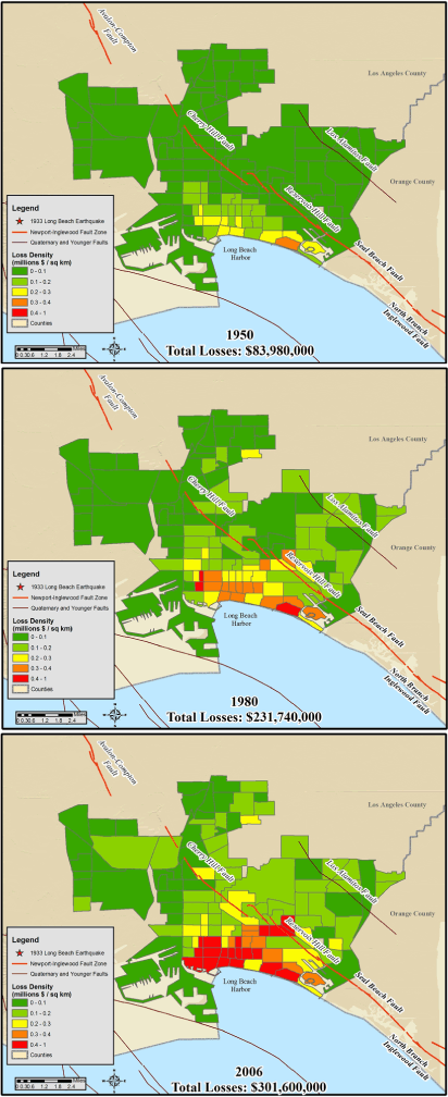
Spatial distribution of estimated total building damage by decade, divided by the area of each census tract, for the M_w 6.4 Long Beach ground motions. The latitude and longitude bounds of this map are 33.7° to 33.9°, and −118.3° to −118°, respectively.

Magnitude Dependence

Figure 8 presents the temporal variation in total direct economic loss as a function of earthquake magnitude. In this paper direct economic losses refer to capital stock losses including damages to structures, nonstructural inventory, business inventory, and building contents. For instance, if these scenarios had occurred in 2006, the total capital stock losses would have ranged from $131–$781 million (2002 costs) for a M_w 6.0 or M_w 7.2 event, respectively. Between M_w 6.0 and M_w 7.2, earthquake magnitude amplifies losses 17%. The rate of loss increases significantly as a function of exposure density and/or magnitude. The results in Figures 6, 7, and 8, including the flattening of the curves from 1990 onward, show that the risk increases with respect to earthquake magnitude and increased exposure density as the building stock grows over time, and the implementation of improved seismic building codes since the 1970s. The reliance on the current assessor's database (which only contains information on the current buildings) meant we could not readily model building stock replacement, and that our modeling of earlier exposures will certainly underestimate risk as those buildings removed from the building stock will not be reflected in the results.

Figure 8.

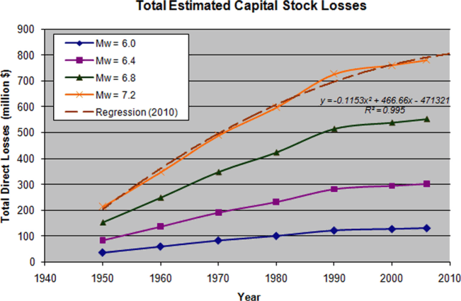
Total estimated direct economic losses by earthquake scenario and decade. The regression equation was determined based on the temporal variation is losses due to a M_w 7.2 earthquake (dashed orange), that was assumed to occur in 2010 in the study area.

Discussion and Conclusions

In general, the spatial distribution of total exposure (building value) and direct economic losses computed by Hazus-MH MR3 indicates that the amount of damage is not limited to a single factor but to a combination of influences including proximity to the historical fault rupture (Figure 5) and density of construction (Figure 6), as well as amount of dollar exposure (Figure 7). Thus census tracts in the central and southern portions of the study area are predicted to suffer relatively greater losses with respect to the four earthquake scenarios analyzed, as would be expected.

The results demonstrate that software such as Hazus-MH can be used effectively to estimate historical economic losses due to earthquakes, and thus provide a means of forecasting potential losses based on temporal variation of damages with respect to a given earthquake scenario. This study predicts damage and losses in the Long Beach area of approximately $840 million in 2002 dollars if an earthquake of M_w 7.2 with the same source parameters as the 1933 event were to have occurred in 2010. The loss estimates would be higher if we used 2008 costs and lower if this analysis had taken into account design improvements made to existing structures. This could be accomplished by integrating model building types that represent seismically retrofitted structures into the methodology. For instance, Kircher et. al. (2006) also used Hazus-MH MR1 technology to estimate damage and losses likely to occur in a 19-county Northern California study region due to a repeat of the 1906 San Francisco earthquake. Rather than completely replacing the structural inventory, they updated the default inventory mapping scheme by replacing it with custom mapping schemes that describe real combinations of model building types in their study area, modified the default building properties to more closely represent the most vulnerable building types, and added new retrofitted model types. Their study area was much larger (about ten times as many buildings) and the scenario earthquake ground motions were stronger than those of the study discussed in this paper, which helps to explain the larger loss estimates generated ($90–$120 billion).

The results from both our study and Kircher et. al. (2006) indicate some of the ways the Hazus-MH modeling suite can be customized to better represent local conditions. While the study discussed in this paper yields better loss estimates than would be possible using Hazus-MH with default national level datasets, there are still several additional issues worth noting.

First, the calculations are based on a single attenuation relationship, while several equally viable ground motion models could have been utilized that would have produced different loss estimates (Field et. al. 2005). Most significantly, next generation attenuation (NGA) relations should be tested on the same datasets and the results compared (Campbell and Bozorgnia 2006).

Second, qualitative estimation of potential losses based on historical structural inventories cannot consider the full range of possibilities of effects on losses in the future. Potential losses will be directly impacted by economics (i.e., rate of inflation), construction (i.e., building counts, evolution of seismic codes, structural designs, and construction materials), and population growth. Present-day highly vulnerable building types such as soft-story apartment buildings, as well as newly retrofitted structures could be accommodated by developing customized mapping schemes within Hazus. Also, detailed mapping of the damage and losses incurred in 1933 would provide additional ground-truth with which to compare the results.

Third, the variations in the seismic building codes for each decade and the possible range of losses which could be computed using different vulnerability relationships could be explored in order to determine the reliability of the estimates computed in this study.

Fourth, this application holds site effects constant for the entire study area, namely National Earthquake Hazards Reduction Program (NEHRP) Site Class D. The addition of a spatially explicit local soil map (see Lam et. al. 2007 for an example) would allow a more precise prediction of damages and losses. In addition, these results could be augmented with future analyses that also take rupture directivity into account.

Lastly, the temporal variation in fatalities could be more accurately assessed provided the population counts and demographic information for each decade were integrated into the study region datasets for the latest release of the Hazus software, Hazus-MH MR4. For example the Comprehensive Data Management System (CDMS) version 2.5 tool developed by FEMA allows updating of pre-aggregated census data as well as structural inventory information. However, significant pre-processing and organization of demographic information would be required by Hazus-MH MR4 in decade increments to augment this particular study.

Thus, in the future, this study could be augmented by updating the loss estimates to current values, integrating an accurate soil condition map of the study area, and inserting updated demographics within each Hazus-MH MR3 decade (study region dataset) in order to predict the social impact and improve the structural loss estimates of these scenarios for Long Beach.

Footnotes

Acknowledgments

This study was supported by the Human and Social Dynamics Program of the National Science Foundation, Washington, D.C. (Grant No. CMS-0433376). Special thanks to Robert L. Nigbor for valuable review comments.

References

Abrahamson

N. A.

, and Silva

, 1997. Empirical response spectral attenuation relations for shallow crustal earthquakes, Seismological Research Letters 68, 94–127.

American Society of Civil Engineers (ASCE), 2003. 6th U.S. Conference and Workshop on Lifeline Earthquake Engineering, 10–13 August 2003, Long Beach, CA.

American Society of Civil Engineers (ASCE), 2005. Minimum Design Loads for Buildings and Other Structures, Standard ASCE/SEI 7-05, including Supplement 1, Reston, VA.

Barrows

A. G.

, 1974. A Review of the Geology and the Earthquake History of the Newport-Inglewood Structural Zone, Southern California, California Division of Mines and Geology Special Report 114, Sacramento, CA.

Benioff

, 1938. The determination of the extent of the faulting application to the Long Beach earthquake, Bulletin of the Seismological Society of America, 28, 77–84.

Boore

D. M

, Joyner

W. B.

, and Fumal

T. E.

, 1997. Equations for estimating horizontal response spectra and peak acceleration from western North American earthquakes: A summary of recent work, Seismological Research Letters 68, 128–153.

Bryant

W. A.

(compiler), 2005. Digital Database of Quaternary and Younger Faults from the Fault Activity Map of California, Version 2.0, California Geological Survey Web page, http://www.consrv.ca.gov/CGS/information/publications/QuaternaryFaults_ver2.htm, accessed May 2009.

California Division of Mines and Geology, 1988. Planning Scenario for a Major Earthquake on the Newport-Inglewood Fault Zone, Special Publication 99, Sacramento, CA.

Campbell

, W. 1976. A Note on the Distribution of Earthquake Damage in Long Beach, 1933. Bulletin of the Seismological Society of America 66(3), 1001–1005.

10.

Campbell

K. W.

, and Bozorgnia

, 2003. Updated near-source ground motion (attenuation) relations for the horizontal and vertical components of peak ground acceleration and acceleration response spectra, Bulletin of the Seismological Society of America 93, 314–331.

11.

Campbell

K. W.

, and Bozorgnia

, 2006. Campbell-Bozorgnia next generation attenuation (NGA) relations for PGA, PGV and spectral acceleration: a progress report, Paper No. 906, Proceedings of the 8th U.S. National Conference on Earthquake Engineering, 18–22 April 2006, San Francisco, CA.

12.

City of Los Angeles, 2008. Los Angeles International Earthquake Conference (IECLA), 12–14 November, 2008, Los Angeles, CA.

13.

Comerio

M. C.

, Landis

J. D.

, Firpo

C. J.

, and Monzon

J. P.

, 1996. Residential Earthquake Recovery, California Policy Seminar, University of California, Berkeley.

14.

Dolan

J. J.

, Sieh

, Rockwell

T. K.

, Yeats

R. S.

, Shaw

, Suppe

, Huftile

G. J.

, and Gath

E. M.

, 1995. Prospects for larger or more frequent earthquakes in the Los Angeles metropolitan region, Science 267, 199–205.

15.

Earthquake Engineering Research Institute (EERI), 2006. 100th Anniversary Earthquake Conference Commemorating the 1906 San Francisco Earthquake, 18–22 April 2006, San Francisco, CA.

16.

Eguchi

, Chang

S. E.

, and Seligson

, 1998. Direct economic losses in the Northridge earthquake: A three-year post-event perspective, Earthquake Spectra 14, 245–264.

17.

EQE International, Inc., 1997. The Northridge Earthquake of January 17, 1994: Report of Data Collection and Analysis, Part B: Analysis and Trends, prepared for the California Governor's Office of Emergency Services, May 1997, Irvine and Pasadena, California.

18.

Ethington

P. J.

, Kooistra

A. M.

, and DeYoung

, 2000. Los Angeles County Union Census Tract Data Series, 1940-1990, User's Guide, Version 1.01, University of Southern California, Los Angeles.

19.

Federal Emergency Management Agency (FEMA), 2004. NEHRP Recommended Provisions for Seismic Regulations for New Buildings and Other Structures, FEMA 450-I, 2003 edition Washington, D.C.

20.

Federal Emergency Management Agency (FEMA), 2007. Multi-hazard Loss Estimation Methodology Earthquake Model, Hazus-MH MR3 User's Manual, Mitigation Division, Washington, D.C., 290 pp.

21.

Federal Emergency Management Agency (FEMA), 2008a. Multi-hazard Loss Estimation Methodology Earthquake Model, Hazus-MH MR3 Technical Manual, Mitigation Division, Washington, D.C.

22.

Federal Emergency Management Agency (FEMA), 2008b. Hazus-MH Estimated Annualized Earthquake Losses for the United States, FEMA 366, Mitigation Division, Washington, D.C.

23.

Field

E. H.

, Seligson

H. A.

, Gupta

, Jordan

T. H.

, and Campbell

K. W.

, 2005. Loss estimates for Puente Hills blind-thrust earthquake in Los Angeles, California, Earthquake Spectra 21, 329–338.

24.

Frankel

A. D.

, Peterson

M. D.

, Mueller

C. S.

, Haller

K. M.

, Wheleler

R. L.

, Leyendecker

E. V.

, Wesson

R. L.

, Harmsen

S. C.

, Cramer

C. H.

, Perkins

D. M.

, and Rukstales

K. S.

, 2002. Documentation for the 2002 Update of the National Seismic Hazard Maps, USGS Open-File Report 02-420, Reston, VA.

25.

Grant

L. B.

, Waggoner

J. T.

, Rockwell

T. K.

, and Stein

C. V.

, 1997. Paleoseismicity of the north branch of the Newport-Englewood fault zone in Huntington Beach, California, from cone penetrometer test data, Bulletin of the Seismological Society of America 87, 277–293.

26.

Hauksson

, 1987. Seismotectonics of the Newport-Inglewood fault zone in the Los Angeles Basin, Southern California, Bulletin of the Seismological Society of America 77, 539–561.

27.

Hauksson

, and Gross

, 1991. Source parameters of the 1933 Long Beach earthquake, Bulletin of the Seismological Society of America 81, 81–98.

28.

Housner

G. W.

, 2002. Historical view of earthquake engineering, in International Geophysics ( Lee

W. H. K.

, Kanamori

, Jennings

P. C.

, Kisslinger

, Eds.) Academic Press 81 Part A, 13–18.

29.

ImageCat and ABS Consulting, 2006a. Data Standardization Guidelines for Los Estimations – Populating Inventory Databases for Hazus^®-MH MR1, prepared for the California Governor's Office of Emergency Services by ImageCat, Inc., Long Beach, CA and ABS Consulting, Irvine, CA.

30.

ImageCat and ABS Consulting, 2006b. How to use the building inventory replacement tool (BIRT) for a Hazus^®-MH earthquake (EQ) study region (SR), Appendix C, in Data Standardization Guidelines for Los Estimations – Populating Inventory Databases for Hazus^®-MH MR1, prepared for California Governor's Office of Emergency Services by ImageCat, Inc., Long Beach, CA and ABS Consulting, Irvine, CA.

31.

ImageCat and ABS Consulting, 2006c. Data Standardization Guidelines for Los Estimations – Populating Inventory Databases for Hazus^®-MH MR1: Pilot Studies Report – Los Angeles County, prepared for the California Governor's Office of Emergency Services by ImageCat, Inc., Long Beach, CA and ABS Consulting, Irvine, CA.

32.

Kircher

C. A.

, Seligson

H. A.

, Bouabid

, and Morrow

G. C.

, 2006. When the Big One strikes again: Estimated losses due to a repeat of the 1906 San Francisco earthquake, Earthquake Spectra, 22, S297–S339.

33.

Lam

, Swift

, and Wilson

J. P.

, 2007. A Digital Soil Map for the Green Visions Plan for 21^st Century Southern California Study Area, Tech. Rep. No. 5, GIS Research Laboratory, University of Southern California, Los Angeles.

34.

Los Angeles County, 2010a. Office of the Assessor Web site, http://assessor.lacounty.gov/extranet/default.aspx, accessed December 2011.

35.

Los Angeles County, 2010b. Office of the Assessor property search Web page, http://maps.assessor.lacounty.gov/mapping/viewer.asp, accessed December 2011.

36.

Martel

R. R.

, 1965. Earthquake damage to Type III buildings in Long Beach, 1933, in Earthquake Investigations in the Western United States 1931–1964, U.S. Coast and Geodetic Survey Publication 41–2, 213–222

37.

Meehan

J. F.

, 1972. History of earthquake code in California, in final report to the state legislature by the Joint Committee on Seismic Safety, Schoolhouse Section, California Office of Architecture and Construction.

38.

Occupational Safety & Health Administration (OSHA), 2009. Standard Industrial Classification (SIC) division structure, Web site, U.S. Department of Labor, http://www.osha.gov/pls/imis/sic_manual.html, accessed December 2011.

39.

Olsen

R. A.

, 2003. Legislative politics and seismic safety: California's early years and the “Field Act”, 1925–1933, Earthquake Spectra 19, 111–131.

40.

Sadigh

, Chang

C. Y.

, Egan

J. A.

, Makdisi

, and Youngs

R. R.

, 1997. Attenuation relationships for shallow crustal earthquakes based on California strong motion data, Seismological Research Letters 68, 180–189.

41.

Southern California Earthquake Research Center (SCEC), 2009. Long Beach Earthquake: 70th Anniversary, Web page, http://www.scec.org/education/030310longbeach.html, accessed June 2009.

42.

Spudich

, Joyner

W. B.

, Lindh

A. G.

, Boore

D. M.

, Margaris

B. M.

, and Flecher

J. B.

, 1999. SEA99: A revised ground motion prediction relation for use in extensional tectonic regimes, Bulletin of the Seismological Society of America 89, 1156–1170.

43.

Strand

D. R.

, 1984. Code development between 1927 and 1980, in Proceedings of the 1984 Convention, Structural Engineers Association of California, Monterey, October 18–20, Sacramento, CA.

44.

Swift

J. N.

, Nguyen Le

, and Wilson

J. P.

, 2009. Data Standardization of Los Angeles County Assessor 2006 Structural Inventory of Long Beach, CA, Tech. Rep. No. 11, GIS Research Laboratory, University of Southern California, Los Angeles.

45.

Tatalovich

, and Wilson

J. P.

, 2007. Reconstructing Spatio-Temporal Patterns of Social Vulnerability in Los Angeles from 1940 to 2000, unpublished.

46.

Wells

D. L.

, and Coppersmith

K. J.

, 1994. New empirical relationships among magnitude, rupture length, rupture width, rupture area, and surface displacement Bulletin of the Seismological Society of America 84, 974–1002.

47.

Yerkes

R. F.

, McCulloh

T. H.

, Schoellhamer

J. E.

, and Vedder

J. G.

, 1965. Geology of the Los Angeles Basin, California: An introduction, U.S. Geological Survey Professional Paper 420-A, Reston, VA.

48.

Ziony

J. I.

, and Yerkes

R. F.

, 1985. Evaluating earthquake and surface-faulting potential, in Evaluating Earthquake Hazards in the Los Angeles Region, U.S. Geological Survey Professional Paper 1360 ( Ziony

J. I.

, ed.), Reston, VA, 43–91.

49.

Ziony

J. I.

, Evernden

J. F.

, Fumal

T. E.

, Harp

E. L.

, Hartzell

S. H.

, Joyner

W. B.

, Keefer

D. K.

, Spudich

P. A.

, Tinsley

J. C.

, Yerkes

R. F.

, and Youd

T. L.

, 1985. Predicted geologic and seismologic effects of a postulated magnitude 6.5 earthquake along the northern part of the Newport-Inglewood zone, in Evaluating Earthquake Hazards in the Los Angeles Region, U.S. Geological Survey Professional Paper 1360 ( Ziony

J. I.

, ed.), Reston, VA, 415–441.