Ground Motion Selection for Liquefaction Evaluation Analysis of Earthen Levees

Abstract

Guidelines for selecting ground motions for liquefaction evaluation analysis of earthen levees are proposed. These guidelines were developed based on results from dynamic analyses of characteristic earthen levee cross sections using a wide range of ground motions (~1,500). The effect of a number of ground motion parameters on the dynamic response of the levees in terms of liquefaction susceptibility was studied, and the parameters that correlated best to the response were identified. For the liquefaction triggering evaluation, the mean period of the ground motion (T_m) is best correlated to the cyclic stress ratio (CSR). Regression relationships between CSR and T_m are proposed for a series of levee types and shaking intensities.

Introduction

Ground motion selection is a challenging engineering problem since the variability in ground motion characterization is, in part, due to the complexity of the mechanisms that result in a seismic event taking place, the path of the earthquake, and the soil conditions from the origin of the seismic event to the location of interest. In seismic slope stability analyses the single most important input parameter is the ground motion (Bray 2007, Bray and Travasarou 2007). Recent studies (Athanasopoulos-Zekkos 2008) showed that the variability in seismic levee response due to the selection of a wide range of ground motions was much higher than the variability in response due to varying soil stratigraphy and levee geometry. Robust estimates on the seismic vulnerability of earthen levees are needed because the government is moving toward reassessing the condition of our nation's flood protection systems. Recent studies (URS 2007) concluded that there is a 0.5% chance per year, approximately, of an earthquake event occurring in Northern California that would cause more levee breaches within the Sacramento-San Joaquin River Delta than could be repaired within a 12-month time window, in time for the annual high flood water level. Levees along the Mississippi River could also be compromised due to a seismic event in the New Madrid Seismic Zone. The effect of key ground motion parameters on the dynamic response of earthen levees has been studied by Athanasopoulos-Zekkos (2010) and the results from that study are used here to develop regression models to help in the development of ground motion selection guidelines for liquefaction triggering evaluation of earthen levees.

Dynamic Response of Levees

The seismic vulnerability of levees is associated with a loss of freeboard due to liquefaction of the levee or foundation soils. Unfortunately, there is little-to-no guidance as to how to evaluate the seismic vulnerability of levees. A systematic study of the dynamic response of three characteristic levee cross sections for Central California was conducted by Athanasopoulos-Zekkos (2008) and a simplified procedure for the evaluation of the seismic vulnerability of earthen levees was proposed. However, there are several instances when more advanced dynamic analyses are needed, such as for levee cross sections that are marginally safe or unsafe according to the simplified procedure or levee cross sections that have a different soil stratigraphy from the three sections included in the study. The most critical input parameter for these dynamic analyses is the acceleration time history. By using large numbers of ground motions (i.e., hundreds or thousands) the average response, as well as the variability of the response, can be evaluated. However, in common engineering practice a small number (typically seven) of acceleration time histories are used to study the seismic response of earthen structures. It is therefore difficult to capture the average response and its variability without understanding which ground motion parameter affects it the most. Furthermore, depending on which parameters have been selected to study the dynamic response of an earthen structure the most influential ground motion parameters in terms of the response will be different.

Athanasopoulos-Zekkos (2008) used a wide range of ground motions (~1,500) to study and develop statistically stable estimates of the dynamic response for three different levee sites and also to provide insight toward the effects of ground motion selection on the dynamic response of earthen levees. Equivalent-linear, 2-D finite element dynamic analyses were performed using QUAD4M (Hudson et al. 1994). Equivalent-linear models and nonlinear models can both be used successfully for site response analyses. There is, however, always the need for engineering judgment in selecting the input parameters and interpreting the results. Equivalent-linear models produce reasonable results for problems where strain levels remain low, either due to stiff soil profiles or relatively weak ground motions, whereas nonlinear models are likely to be more accurate for problems where the induced shear stresses approach the available shear strength of the soil, and thus the shear strains are large. Shear strains computed in the analyses presented in this study did not exceed 3%. The ground motions were selected from the Pacific Earthquake Engineering Research Center, NGA strong motion database (PEER 2007). The recordings that were selected satisfied the following criteria:

Moment magnitude (M_w) = 5.5 to 7.7

Distance of site of recording from epicenter (EpiD) = 20 km to 110 km

Preferred V_S₃₀ > 180 m=sec (~600 ft/sec)

Peak ground velocity (PGV) < 100 cm=sec and peak ground displacement (PGD) < 100 cm

Additional details on the selection of ground motions and levee cross sections are presented in Athanasopoulos-Zekkos (2008 and 2010). The selected ground motions were scaled to match peak ground acceleration input levels (PGA_input) of 0.1 g, 0.2 g, 0.3 g, and 0.4 g. The only way the ground motion records were modified for this study was by scaling the entire acceleration time history amplitude by a given factor, so as to match the prescribed PGA_input. The maximum amplitude scaling factors were constrained within a range of 0.5 to 2. Krinitszky and Chang (1979) recommended that the scaling factor should be kept as close to 1 as possible, and always between 0.25 and 4.0. Vanmarcke (1979) noted that simple amplitude scaling fails to account for other important characteristics (e.g., frequency content, duration, etc.) and therefore recommended that limits to the scaling factor should be related to the type of problem to which the resulting motion is to be applied. For example, for liquefaction, where duration and cycles of loading combined with intensity are important, scaling factors in the range of 0.5 to 2.0 should be used. Watson-Lamprey and Abrahamson (2006) found that limits to scaling factors are appropriate if the candidate time series are selected based only on the magnitude, distance, and site condition; however if more specific selection criteria that are based on additional properties of the ground motion are used (e.g., frequency content and wave form), then a wider range of scaling factors can be used. Since the original selection of ground motions was based only on moment magnitude (M_w), EpiD, and site conditions (V_S₃₀), the scaling factors were constrained to a range from 0.5 to 2. All motions that were recorded at the surface of a soil deposit were deconvolved before being assigned as input ground motions. This was automatically performed by QUAD4M prior to all analyses.

The three typical levee cross sections analyzed are representative of three areas in California: Stockton, West Sacramento, and Marysville. These are denoted as Levee Types A, B, and C, respectively, and are among the sites under study as part of the Urban Levee Project of the California Department of Water Resources. Figure 1a shows the geometry and soil stratigraphy for the three levee types. The depth to the transmitting base for the three levee cross sections was determined based on studies performed by URS Corp. for the Delta Risk Management Strategy Project (URS 2007) and for the Urban Levee Geotechnical Evaluations (Scott Shewbridge, personal communication). Generally, it is preferred to establish a clear boundary indicated by a high impedance ratio resulting from a change in the shear wave velocity between two layers. This is relatively straightforward when bedrock, or some form of rock or very stiff soil is encountered at some elevation. In this case however, due to the depositional environment of California's Central Valley, the soil deposits extend for many hundreds of feet, stiffening progressively with increased depth making it impractical to extend the finite mesh all the way to “bedrock.” Instead, it was decided to cut off the finite mesh at the elevation where the soil deposits reach a shear wave velocity of 1,200 ft/sec (Figure 1b), and to model a half-space below that elevation. In all three cases this meant including the upper layers of the Pleistocene deposits.

Figure 1.

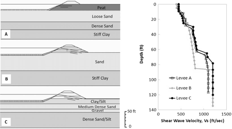
(a) Levee geometry and soil stratigraphy and (b) corresponding shear wave velocity profile for Levees A (Stockton), B (West Sacramento), and C (Marysville).

Shear stresses were computed only at a select number of locations for each of the three levee types to reduce the computational time required by QUAD4M. Furthermore, the results are reported at select elevations at each of the studied locations. Elevation values (in feet) are relative to the channel bed bottom (elevation reference = 0 ft).

The computed shear stresses for several vertical sections, as shown in Figure 2, across the levee sites were then normalized by the in-situ vertical effective stress, to produce calculated values of equivalent cyclic stress ratio (CSR_eq; Seed and Idriss 1971) for all PGA_input levels, all three levee types, and all locations studied, as shown in Equation 1:

C S R_{e q} = \frac{τ_{c y c l i, e q}}{σ'_{v}} = 0.65 \frac{τ_{c y c l i, \max}}{σ'_{v}}

(1)

where τ_{cyclic, max} is the actual induced maximum shear stress, and σ _v ^′ is the vertical effective stress at the respective elevation.

Figure 2.

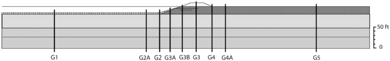
Locations of computed shear stress and cyclic stress ratio profiles for Levee A.

From the CSR values calculated at the finite number of locations, a 2-D CSR profile was established along the levee cross sections. Figure 3 shows an example of the results for Levee A for a PGA_input of 0.2 g.

Figure 3.

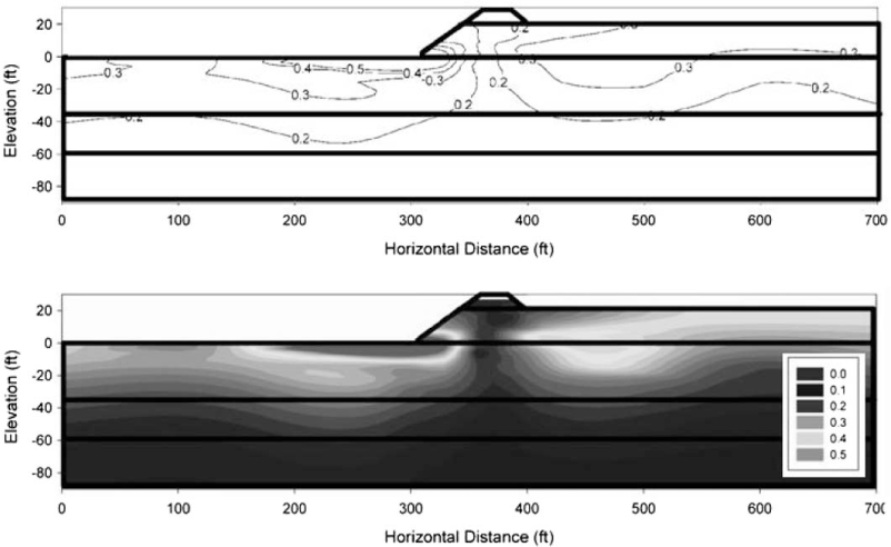
CSR_eq contours for Levee A with a PGA_input of 0.2 g.

Ground Motion Parameter Analyses

The created CSR_eq profiles, which show variations in space and elevation along a levee type cross section, represent the median values of a large distribution of dynamic response resulting from the use of the ~1,500 ground motions. It was found that variability in the CSR values results from variability in the ground motions rather than the soil stratigraphy (Athanasopoulos-Zekkos 2008).

A number of parameters have been studied with respect to their correlation to CSR. These include the moment magnitude, M_w, the significant duration, D_5–95, the spectral acceleration at the site period, Sa @T_s, the spectral acceleration at the degraded site period, Sa @ 1.5*T_s, and the mean period of the ground motion, T_m (Rathje et al. 1998). The ground motion parameter that most strongly correlated with the CSR variability was found to be the mean period of the ground motion (Athanasopoulos-Zekkos 2010). This trend is expected since seismically induced soil shear stresses are particularly dependent on a ground motion's frequency content (e.g., Idriss and Boulanger 2008). However, to develop specific selection criteria, regression analyses have to be performed to describe the relationship between CSR and T_m.

Problem Background and Methodology

For each levee type, the cross section profile locations to be analyzed were chosen to reflect the conditions (1) at the free-field (i.e., far from the levee, Location G1), (2) at the levee toe (Location G2), and (3) at the levee crest (Location G3). In addition, Levee A has an asymmetric geometry where the waterside toe and the landside toe have different elevations; therefore for Levee A the analysis was also performed at the landside toe (Location G4).

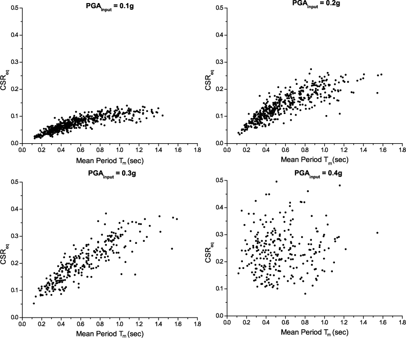
The analysis was carried out for four sets of ground motions, as mentioned before, representing input peak ground accelerations (PGA_input) of 0.1 g (549 ground motions), 0.2 g (459 ground motions), 0.3 g (284 ground motions), and 0.4 g (262 ground motions). For each set of PGA values, levee type, and location, the CSR data points were plotted vs. T_m for all elevations. The following first observations can be made:

The CSR values increase as the mean period increases, regardless of the site's natural period (Figures 4 and 5).

The correlation between CSR and T_m becomes less pronounced as PGA increases (Figure 4). This may be due to nonlinearity effects (e.g., higher shear strains, a nonlinear relationship between stress and strain) that are more pronounced at high accelerations, but are not captured by the equivalent-linear analyses performed herein.

The correlation between CSR and the ground motion mean period becomes less pronounced with decreasing depth, as reflected in Figure 5. This is expected since the ground motion characteristics (e.g., T_m) change as the ground motion propagates through the soil layers and reaches the surface. Therefore the T_m of the input ground motion no longer correlates well with the shear stresses produced near shallower soil layers.

For the case of the asymmetric geometry at Levee A where the waterside toe (Location G2) and the landside toe (Location G4) have different elevations, the analyses (e.g., Figure 3) showed that the critical (high) values of CSR occurred at Location G2, and therefore Location G4 at Levee A will not be included in the analyses.

Regression Analysis and Choice of Best-Fit Equation Forms

A number of functions were tested for the best fit of the scatter points. The criteria for the function that best fit the data included comparison of residuals (defined as the percentage difference between the fitted and actual values, as compared to the actual values) and root mean square error (RMSE) values resulting from different fit functions.

Figure 4.

CSR values vs. mean period (T_m) for Levee A at Location G1 with data shown only for 87 ft from the channel bottom.

Figure 5.

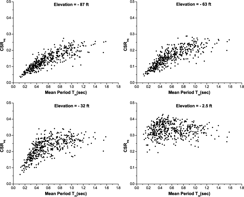
CSR values vs. mean period (T_m) for Levee A with a PGA_input of 0.2 g at Location G1, with data shown for representative elevations of −2.5 ft, −32 ft, −63 ft, and −87 ft from the channel bottom.

The function that provided the best fit was the power function. Two forms of this function were analyzed, as shown in Equations 2 and 3, representing Form #1 and Form #2, respectively:

C S R_{e q} = a \cdot T_{m}^{b} + c

(2)

C S R_{e q} = a \cdot T_{m}^{b}

(3)

where a, b, and c are the regression coefficients to be determined.

Form #2 reflects an intercept of zero on the CSR axis corresponding to a mean period of zero. However, applying the equation of Form #1, which implies an intercept value, resulted in slightly lower RMSE values (1–8% better than Form #2). Lower values of RMSE reflect a smaller difference between the actual observed values and the estimated fit values.

R-square, by definition, theoretically ranges from 0–1. A higher R-square value implies a better fit. Values of R-square are very low at shallow depths, irrespective of the fit form used, which reflects the weaker correlation between CSR and T_m as the ground motion propagates through more soil layers on its way to the surface.

Figure 6 shows the difference in the RMSE and R-square values based on the use of the two different power equation forms at Levee A for a PGA_input of 0.2 g at Location G1. The range and variation with elevation of the R-square values (Figure 6b) is also similar for all three levee cross sections, locations, and PGA_input values. The RMSE values (Figure 6a), however, increase with higher PGA_input values.

Figure 6.

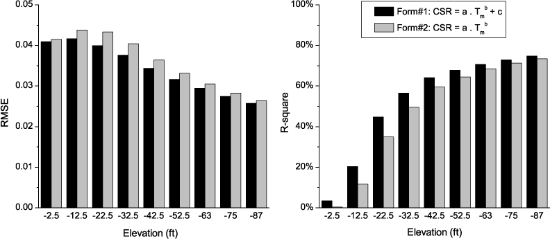
(a) RMSE and (b) R-square values for both Forms #1 and #2 at Levee A for a PGA_input of 0.2 g at Location G1.

Figure 7 shows the percentage residuals of CSR for both Forms #1 and #2 at three elevations in Levee A for a PGA_input of 0.2 g at Location G1, calculated as shown in Equation 4:

R e s i d u a l (%) = \frac{(C S R_{c o m p u t e r} - C S R_{f i t})}{C S R_{c o m p u t e r}}

(4)

where CSR_computed is the computed cyclic stress ratio value and CSR_fit is the value obtained from the fit equations.

Figure 7.

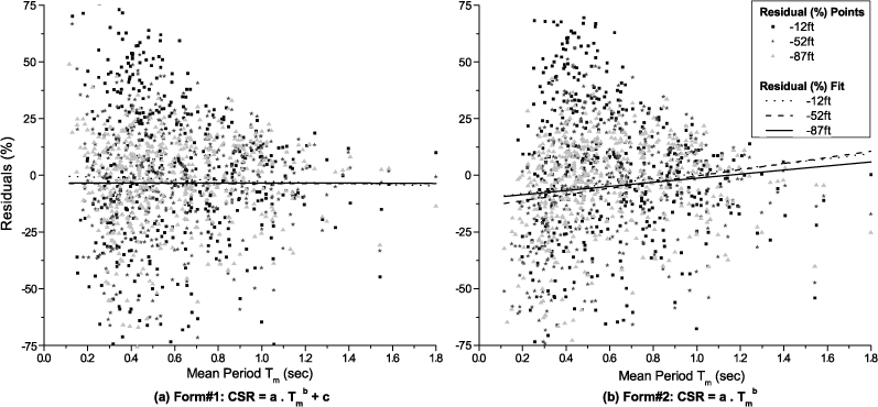
Comparison of the percentage residuals for both (a) Form #1 and (b) Form #2 at three representative elevations in Levee A, for a PGA_input of 0.2 g at Location G1.

Figure 8 shows a comparison of the power function fit using both Equation Forms #1 and #2 at Levee A for a PGA_input of 0.2 g at Location G1 at representative elevations of −63 ft and −87 ft. The results shown in these figures are representative of all three levee types and locations.

Figure 8.

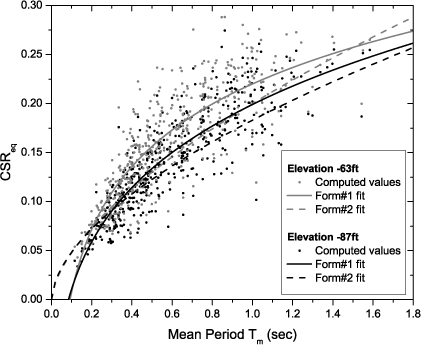
Comparison of the fit for both Forms #1 and #2 at elevations of −63 ft and −87 ft for Levee A with a PGA of 0.2 g for Location G1.

The majority of the T_m values are in the range where Equation Form #1 and Form #2 seem to overlap (e.g., in Figure 8, more than 95% of T_m values corresponding to a PGA_input of 0.2 g are between 0.2 and 1.2 sec). Based on the above, it can be noted that although Equation Form #1 has a slightly better fit to the data than Equation Form #2, it requires setting a minimum limit on the T_m values that can be used, since Form #1 fit does not pass through the origin of the plot. Because of this constraint, and since the R-square and RMSE indicators of Form #2 do not differ substantially, the analysis of the data was carried out based on Form #2, which represents a relationship between the CSR_eq values and the mean period (T_m) of the ground motions used in the form CSReq = a^*T_m^b, as previously shown in Equation 3. It is also worth noting that the results from the analyses with a PGA_input of 0.4 g were not used in the regression because it was observed that, due to nonlinearity effects, the correlation between CSR and T_m was very weak.

Relationship of Best Fit Parameters with Elevation

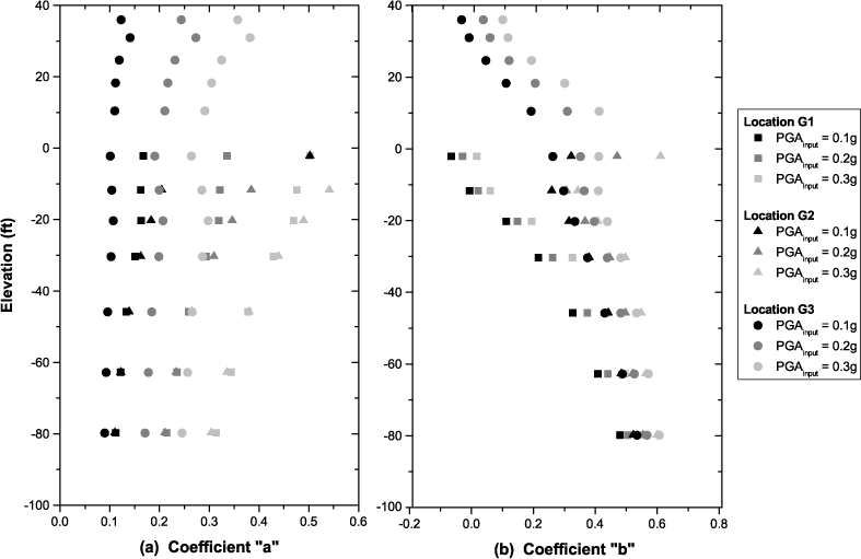
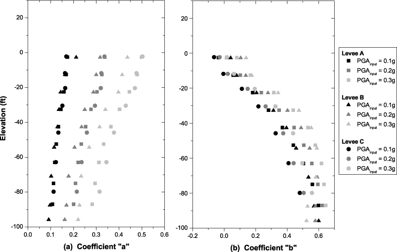
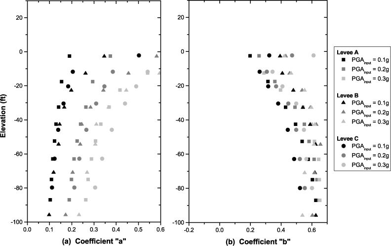
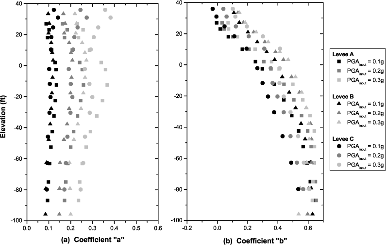
The terms a and b are coefficients that vary with each levee type, location, and elevation. In order to highlight the effect of levee geometry on the results, the variation of the coefficients a and b with elevation at each of the Levees A, B, and C, and for various locations and PGA levels is shown in Figures 9 through 11.

Figure 9.

Variation of Equation Form #2 coefficients a and b with elevation, in Levee A, for all locations and PGA levels.

Figure 10.

Variation of Equation Form #2 coefficients a and b with elevation, in Levee B, for all locations and PGA levels.

Figure 11.

Variation of Equation Form #2 coefficient a and b with elevation in Levee C, for all locations and PGA levels.

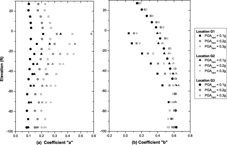
The effect of the different stratigraphy in the three levee types is shown in Figures 12 through 14 where the variation of the coefficients a and b with elevation is plotted at each of the Locations G1, G2, and G3, for all levee types, and PGA levels.

Figure 12.

Variation of Equation Form #2 coefficients a and b with elevation at Location G1, for all levees and PGA levels.

Figure 13.

Variation of Equation Form #2 coefficients a and b with elevation at Location G2, for all levees and PGA levels.

Figure 14.

Variation of Form #2 coefficient a and b with elevation at Location G3, for all levees and PGA levels.

In looking at the parameters that affect the value of the coefficient a, Figures 9a, 10a, and 11a show a strong correlation of this coefficient to PGA_input, irrespective of the levee type. In addition, as PGA_input increases, the scatter in the range of a values increases as well when comparing Locations G1, G2, and G3. Coefficient a values are also clearly affected by the difference in Locations G1, G2, and G3 in the levee cross sections. Figures 12a, 13a, and 14a indicate that coefficient a is not affected by the levee type, and thus the parameters that are considered to affect coefficient a, and that will be included in the development of the regression, will be limited to elevation, PGA_input, and location.

As for coefficient b, it can be noted by observing Figures 9b, 10b, and 11b that the location (i.e., free-field, levee toe, levee crest) has a more pronounced effect than does PGA_input. Furthermore, Figures 12b, 13b, and 14b illustrate that the coefficient b values are even less dependent on the levee type.

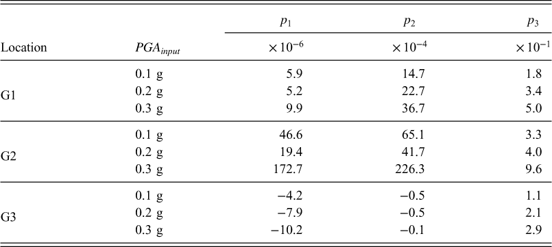
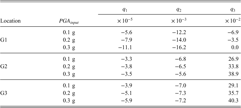
The best regression fit between the coefficients a and b in the equation of Form #2 and elevation was found to have the general polynomial form, shown in Equations 5 and 6, respectively:

a = f (x) = p_{1} \cdot z^{2} + p_{2} \cdot z + p_{3}

(5)

b = f (x) = q_{1} \cdot z^{2} + q_{2} \cdot z + q_{3}

(6)

where z is the elevation in feet, and p₁, p₂, p₃, q₁, q₂, and q₃ are variable coefficients.

The values as well as the variation of the coefficients in Equations 5 and 6 with respect to the different locations and the different PGA_input levels are shown in Tables 1 and 2. This results in separate sets of generalized fitted equations for a and b, one for each levee location (G1, G2, and G3) and each PGA_input level (0.1 g, 0.2 g, and 0.3 g), irrespective of the levee type.

Table 1

Values of p1, p₂, and p₃ for the generalized fit equation of coefficient a for all locations and values of PGA_input

		p ₁	p ₂	p ₃
Location	PGA _input	× 10^-6	× 10^-4	× 10^-1
	0.1 g	5.9	14.7	1.8
G1	0.2 g	5.2	22.7	3.4
	0.3 g	9.9	36.7	5.0
	0.1 g	46.6	65.1	3.3
G2	0.2 g	19.4	41.7	4.0
	0.3 g	172.7	226.3	9.6
	0.1 g	-4.2	-0.5	1.1
G3	0.2 g	-7.9	-0.5	2.1
	0.3 g	-10.2	-0.1	2.9

Table 2

Values of q₁, q₂, and q₃ for the generalized fit equation of coefficient b for all locations and values of PGA_input

		q ₁	q ₂	q ₃
Location	PGA _input	× 10^-5	× 10^-3	× 10^-2
	0.1 g	-5.6	-12.2	-6.9
G1	0.2 g	-7.9	-14.0	-3.5
	0.3 g	-11.1	-16.2	0.0
	0.1 g	-3.3	-6.8	26.9
G2	0.2 g	-3.8	-6.5	33.8
	0.3 g	-3.5	-5.6	38.9
	0.1 g	-3.9	-7.0	29.1
G3	0.2 g	-5.1	-7.3	35.7
	0.3 g	-5.9	-7.2	40.3

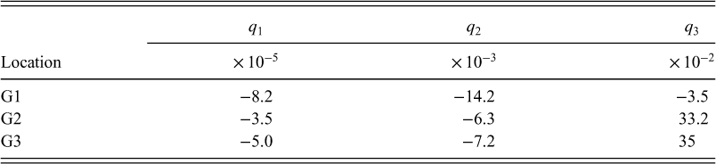
As previously observed by studying Figures 9b through 14b, coefficient b is more dependent on the change in location rather than the change in PGA_input values. Thus, coefficients q₁, q₂, and q₃ can be simplified as per Table 3.

Table 3

Revised values of q₁, q₂, and q₃ for the fit equation of coefficient b at all locations, irrespective of PGA_input

	q ₁	q ₂	q ₃
Location	× 10 ⁵	× 10^-3	× 10 ²
G1	-8.2	-14.2	-3.5
G2	-3.5	-6.3	33.2
G3	-5.0	-7.2	35

Proposed Csr_Eq MODEL

For the final equations describing the relationship between CSR and T_m we can replace a and b in the original Equation Form #2 (Equation 3) where CSR = a^*T_m^b using the generalized fit relationships of a and b as a function of elevation, location, and PGA_input (Equations 5 and 6). This results in the alternative Equation 7 for CSR_eq:

C S R_{e q} = (p_{1} \cdot z^{2} + p_{2} \cdot z + p_{3}) \cdot T_{m} (q_{1} \cdot z^{2} + q_{2} \cdot z + q_{3}) \pm σ_{C S R}

(7)

where z is the elevation in feet, and p₁, p₂, p₃, q₁, q₂, and q₃ are parameters given in Tables 1 and 3 for all three locations and all three shaking intensity levels. σ_CSR is the standard deviation RMSE of CSR_eq.

For elevations of −12.5 ft, −42.5 ft, and −87 ft from the channel bottom, the proposed CSR_eq model fit curves are shown in Figure 15, and the RMSE distribution with elevation for all PGA levels and all locations is shown in Figure 16.

Figure 15.

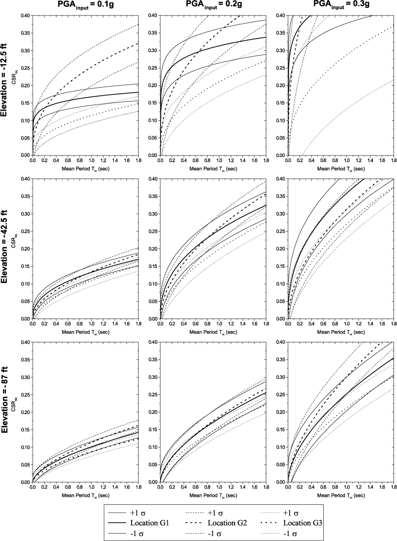
Proposed fit curves for CSR_eq as a function of mean period (T_m) for PGA_input values of 0.1 g, 0.2 g, and 0.3 g, and for elevations of −12.5 ft, −42.5 ft, and −87 ft. CSR is shown at the median value ± one standard deviation RMSE.

Figure 16.

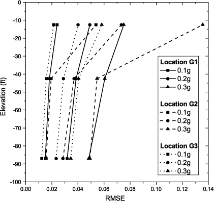
CSR_eq model RMSE variation with elevation for all PGA levels and all locations.

The proposed model and graphs can be used as a ground motion selection criterion for dynamic analyses of earthen levees with regard to liquefaction triggering evaluations. The proposed methodology follows a similar process to the one proposed by Watson-Lamprey and Abrahamson (2006). If the time series, after scaling, are selected such that the time series parameters (i.e., T_m) lead to a median CSR_eq similar to that expected for the design event, then the time series can be expected to give a near-average response for a higher order liquefaction triggering evaluation using a nonlinear soil model. The CSR_eq is therefore used as a proxy for the nonlinear behavior of a more complicated yielding system in guiding the selection of a time series. This approach—defining a proxy for the behavior of a complicated yielding system—has been adopted by other researchers as well (e.g., Haselton 2009). In a typical case, the design ground motion is specified by a response spectrum and an earthquake scenario (M_w, EpiD). The use of the liquefaction model requires an additional parameter: the mean period of the ground motion, T_m. T_m can be estimated using the empirical models and predictive equations proposed by Rathje et al. (1998):

\begin{array}{l} In (T_{m}) = In [C_{1} + C_{2}^{*} (M_{w} - 6) + C_{3}^{*} R] + σ, & f o r M_{w} = 7.25 \end{array}

(8a)

\begin{array}{l} I n (T_{m}) = I n (C_{1} + {1.25}^{*} C_{2} + C_{3}^{*} R) + σ, & for 7.25 < M_{w} < 8.0 \end{array}

(8b)

where for rock C₁, C₂, C₃, and σ are 0.411, 0.0837, 0.00208, and 0.437, respectively, and for soil C₁, C₂, C₃, and σ are 0.519, 0.0837, 0.00190, and 0.350, respectively. R in these relationships is the closest distance to the rupture plane in km.

Figure 17 shows a comparison of the original best fit Form #2 at Levee A, with the developed CSR_eq model equations, which is independent of levee type, for Location G1 and a PGA_input of 0.2 g, for the representative elevations of −87ft, −42.5 ft, and −12.5ft from the channel bottom. As can be seen from the figure, there is very good agreement between the two curves; this is also true for all three levee cross sections, for all cross section locations, and all PGA_input values. The proposed model was also used to compute an equivalent nonlinear shear mass participation factor (r_d) vs. elevation distribution. The results are shown in Figure 18 and are compared to typical r_d values. The curves are in good agreement with the mean values proposed by Cetin et al. (2004), and Idriss and Boulanger (2008) which implies that the proposed model captures the basic characteristics of site response for the three levee profiles.

Figure 17.

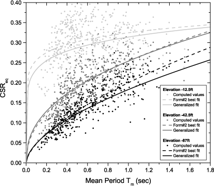
Comparison of Form #2 best fit of CSR_eq vs. T_m at Levee A with the proposed model equation for Location G1, a PGA_input of 0.2 g, at representative elevations of −87 ft, −42.5 ft, and − 12.5 ft.

Figure 18.

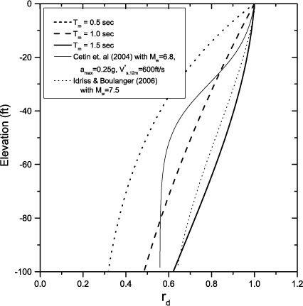
Equivalent r_d results from the proposed model for free-field conditions for a PGA_input of 0.2 g superimposed with lines from recommendations by Cetin et al. (2004), and Idriss and Boulanger (2008).

Finally, the following procedure can be used to select a time series:

Compute the median T_m given the design event parameters using Equations 8a and 8b.

Compute the median CSR_eq for the design event given T_m, using the model in Equation 7 for free-field conditions.

Select candidate ground motion recordings for scaling. This selection can be based on the traditional magnitude and distance bins approach. However, the bins used can be wider than typical.

Scale the PGA of all acceleration time series to match the PGA of the design event ground motion. The scaling factors should be between 0.5 and 2.

Reject records where T_m is not within a half of a standard deviation of its median value, as computed in Step 1.

Calculate the difference between the estimated CSR_eq for the design event (from Step2) and the median CSR_eq expected for each scaled ground motion (Equation 7) and then square the result.

Repeat steps 1–6 for at least three elevation values.

Calculate the root mean square of the differences for the three elevations from Step 7. If both the horizontal components of a record appear on the list, then the component with the lower root mean square is rejected.

Select the record(s) which have the smallest root mean square of differences.

The proposed model can be used for a maximum PGA_input of 0.3 g and for levee cross sections that have similar soil stratigraphy and V_S profiles to Levees A, B, or C.

Conclusions

In dynamic analyses of earthen structures the single most important input parameter is the seismic ground motion (Bray 2007). For the case of earthen levees, their dynamic response was studied using a wide range of ground motions to determine the parameter that best correlates to the cyclic stress ratio (CSR) used in performing liquefaction triggering evaluation. This parameter was found to be the mean period, T_m, of the ground motion (Athanasopoulos-Zekkos 2010). A regression analysis was performed to develop equations that quantitatively describe this correlation. In performing the analyses several observations were made:

(1) The correlation between CSR and T_m is best described using a power function.

(2) The correlation between CSR and T_m becomes less pronounced as PGA increases; this may be due to nonlinearity effects that are more pronounced at high accelerations, but are not captured by the equivalent-linear analyses performed herein.

(3) The trend in CSR increase with mean period values becomes less pronounced at decreasing depths and as the scatter of the values increases. This is expected since the ground motion characteristics (e.g., T_m) change as the ground motion propagates through the soil layers and reaches the surface. Therefore the T_m of the original ground motion no longer correlates strongly with the cyclic shear stresses produced near shallower soil layers.

(4) The main parameters that affect the coefficients used in the proposed equations and therefore the final shape of the CSR vs. T_m curves are: soil stratigraphy, cross section location at levee site (i.e., free-field, levee toe, and levee crest), depth and shaking intensity (described herein by PGA_input). Soil stratigraphy appears to have the smallest effect whereas depth has the largest effect.

(5) The effect of cross section location becomes more pronounced for higher PGA_input values since the topographic effects become more pronounced as well.

A CSR_eq model is proposed to provide selection criteria for ground motions used in site-specific dynamic analyses of earthen levees for liquefaction triggering assessment. This model can be used for a maximum PGA_input of 0.3 g and for levee cross sections that have a similar soil stratigraphy to Levees A, B, or C. The profiles used in these analyses are representative of a wide range of levees. However, if an engineer is faced with a levee section vastly different from the ones presented in this paper, both in terms of stratigraphy and V_S profile, and very strong shaking, the proposed CSR vs. T_m correlation may not be appropriate.

The advantage of using the proposed model is that since the ground motion selection criteria are based on the properties of the scaled ground motion, rather than just selecting time histories based on magnitude, distance, and site, the range of time series typically considered can be significantly broadened, while at the same time the analyses will still lead to an average response of the levee with regard to liquefaction triggering assessment.

References

Athanasopoulos-Zekkos

A. -M.

, 2008. Select Topics on the Static and Dynamic Response and Performance of Earthen Levees, Ph.D. thesis, Department of Civil and Environmental Engineering, University of California, Berkeley.

Athanasopoulos-Zekkos

A. -M.

, 2010. Variability in earthen levee seismic response due to time-history selection, Conference on Recent Advances in Geotechnical Earthquake Engineering and Soil Dynamics, 24–29 May 2010, San Diego, CA.

Bray

J. D.

, 2007. Simplified seismic slope displacement procedures, 4th Annual International Conference on Geotechnical Earthquake Engineering, 25–28 June 2007, Thessaloniki, Greece.

Bray

J. D.

, and Travasarou

, 2007. Simplified procedure for estimating earthquake-induced deviatoric slope displacements, Journal of Geotechnical and Geoenvironmental Engineering 133, 381–392.

Cetin

O. K.

, Seed

R. B.

, Der Kiureghian

, Tokimatsu

, Harder

L. F.

, Kayen

R. E.

, and Moss

R. E. S.

, 2004. Standard penetration test-based probabilistic and deterministic assessment of seismic soil liquefaction potential, Journal of Geotechnical and Geoenvironmental Engineering 130, 1314–1340.

Haselton

C. B.

, 2009. Evaluation of Ground Motion Selection and Modification Methods: Predicting median interstory drift response of buildings, Pacific Earthquake Engeneering Research Center (PEER) Ground Motion Selection and Modification Working Group, Berkeley, CA.

Hudson

, Idriss

I. M.

, and Beikae

, 1994. QUAD4M - A Computer Program To Evaluate the Seismic Response of Soil Structures Using the Finite Element Procedures and Incorporating a Compliant Base, Center for Geotechnical Modeling, Department of Civil and Environmental Engineering, University of California, Davis.

Idriss

I. M.

, and Boulanger

R. W.

, 2008. Soil Liquefaction during Earthquakes, No. MNO-12, EERI Monograph Series, Earthquake Engineering Research Institute, Oakland, CA.

Krinitszky

E. L.

, and Chang

F. K.

, 1979. State of the Art for Assessing Earthquake Hazards in the United States: Specifying peak motions for design earthquakes, Report 7, Misc. Paper S-73-1. U.S. Army Corps of Engineers, WES, Vicksburg, MS.

10.

Pacific Earthquake Engeneering Research Center (PEER), 2007. NGA Strong Motion Database, http://peer.berkeley.edu.nga.

11.

Rathje

E. M.

, Abrahamson

N. A.

, and Bray

J. D.

, 1998. Simplified frequency content estimates of earthquake ground motions, Journal of Geotechnical and Geoenvironmental Engineering 124, 150–159.

12.

Seed

H. B.

, and Idriss

I. M.

, 1971. Simplified procedure for evaluating soil liquefaction potential, Journal of Geotechnical Engineering Division 97, 1249–1273.

13.

URS Corp., 2007. Phase 1 Technical Memorandum Draft 2 - Seismology, Department of Water Resources (DWR) Delta Risk Management Strategy Project, Sacramento, CA, www.water.ca.gov/floodmgmt/dsmo/sab/drmsp/docs/Seismology_TM.pdf.

14.

Vanmarcke

E. H.

, 1979. State of the art for assessing earthquake hazards in the United States: Representation of earthquake ground motion: scaled accelerograms and equivalent response spectra, Report 14, Misc. Paper S-73-1, U.S. Army Corps of Engineers, WES, Vicksburg, MS.

15.

Watson-Lamprey

, and Abrahamson

, 2006. Selection of ground motion time series and limits on scaling, Soil Dynamics and Earthquake Engineering 26, 477–482.

Ground Motion Selection for Liquefaction Evaluation Analysis of Earthen Levees

Abstract

Introduction

Dynamic Response of Levees

Ground Motion Parameter Analyses

Problem Background and Methodology

Regression Analysis and Choice of Best-Fit Equation Forms

Relationship of Best Fit Parameters with Elevation

Proposed CsrEq MODEL

Conclusions

References

Proposed Csr_Eq MODEL