The Temporal and Spatial Dimensions of Price Search: Insights from Matching Household Survey and Purchase Data

Abstract

Price promotions are pervasive in grocery markets. A household can respond to price promotions by effectively cherry-picking through (1) spatial price search across stores and (2) temporal price search across time. However, extant research has analyzed these two dimensions of price search only separately and therefore underestimates both the consumer response to price promotions and the impact of promotions on retail profit. In this article, the authors introduce an integrated analysis of spatial and temporal price search. They seek answers to three questions: First, what are the predictors of household decisions to perform either spatial or temporal price search? Second, how effective are the temporal, spatial, and spatiotemporal price search strategies in obtaining lower prices? and Third, what is the impact of alternative price search strategies on retailer profit? The authors use a unique data collection approach that combines household surveys with observed purchase data to address these questions. Their key results are as follows: Geography (the spatial configuration of store and household locations) and opportunity costs are useful predictors of a household's price search pattern. Households that claim to search spatiotemporally avail approximately three-quarters of the available savings on average. Households that search only temporally save about the same as those that search only spatially. The negative effect of cherry-picking on retailer profits is not as high as is typically believed.

Keywords

consumer search retailing price promotions cherry-picking

Weekly price promotions are a pervasive feature of grocery retailing. A.T. Kearney (2005) estimates that retailers spend from 5% to 10% of their gross revenues in a category on promotions. ACNielsen (2006) estimates that U.S. retailers spent $26.7 billion on promotions in 2005, and promotional sales accounted for roughly 41.5% of total supermarket sales. Given such widespread use and the magnitude of the dollars spent, retail managers and academic researchers have a great interest in understanding how consumers react to retail price promotions and how promotions affect retailer profitability.

The theoretical literature offers two main rationales on why supermarkets offer promotions that are based on heterogeneity in household price search behavior. The first explanation is based on the work of Varian (1980) and relies on household heterogeneity in spatial price search across stores. Some consumers search a lot across stores, whereas others are loyal to their preferred store and do not search. Temporal price promotions arise in equilibrium as a means by which competing retailers offer low prices periodically to attract price-sensitive consumers who search across stores, while charging high prices on average to the high-search-cost consumers who do not search across stores.

The second explanation is based on the work of Conlisk, Gerstner, and Sobel (1984) and Sobel (1984) and relies on household heterogeneity in willingness to search for low prices across time within a store; that is, it relies on heterogeneity in temporal price search. Consumers with low willingness to pay shift their purchases to promotional periods when prices fall below their reservation prices (i.e., they are willing to search for low prices over time), whereas consumers with high willingness to pay purchase at regular prices. Conlisk, Gerstner, and Sobel (1984) and Sobel (1984) model durable goods; in the context of frequently purchased nondurable goods, low-willingness-to-pay customers who wait for the promotion will also stockpile to cover their needs during the nonpromotion periods, thus obtaining a low average price for the product (e.g., Jacobson and Obermiller 1990; Mace and Neslin 2004; Neslin, Henderson, and Quelch 1985). Promotions serve as a price discrimination mechanism; high-willingness-to-pay customers who do not search across time pay high prices on average, whereas low-willingness-to-pay consumers who search across time pay low average prices.

To evaluate the profitability of price promotions, a retailer needs to understand how households cherry-pick in response to price promotions by price searching along both the spatial and the temporal dimensions. However, extant empirical research on price search treats these two dimensions of price search separately. Newman (1977) and Beatty and Smith (1987) provide an extensive review of the literature on spatial price search for durable goods. In recent years, several studies have also focused on understanding spatial price search in grocery markets using either actual purchase or survey data (e.g., Carlson and Gieseke 1983; Fox and Hoch 2005; Putrevu and Ratchford 1997). A parallel stream of empirical literature has focused on the temporal dimension of price search. This literature investigates consumer response to promotions through stockpiling, purchase acceleration, and purchase delays (e.g., Mela, Jedidi, and Bowman 1998; Neslin, Henderson, and Quelch 1985). Here, consumers pay low average prices for goods consumed over time merely by shifting their purchase timing or quantities without doing cross-store shopping.

To our knowledge, no empirical research on price search has investigated household price search jointly along the spatial and temporal dimensions. However, by accounting for only one of the dimensions of price search, we are likely to grossly underestimate the market's response to price promotions and, consequently, its impact on retailer profitability. Given the large body of research on consumer response to price promotions, we believe that this is a significant void in the existing literature. Therefore, we introduce an integrated analysis of spatial and temporal price search in response to price promotions and the impact of such search on retailer profitability.

Our analysis attempts to answer three interrelated research questions. To understand consumers' price search behavior, we need to describe and predict the characteristics of the different search segments so that the retailer can effectively use price search as a basis for segmentation. This leads to our first research question: What are the predictors of different types of consumer price search strategies? To generate predictors of search segment membership, we use an economic model of price search in which households trade off the benefits of price search against the opportunity costs of time for undertaking search (e.g., Putrevu and Ratchford 1997; Urbany, Dickson, and Kalapurakal 1996). We also use several household characteristic and attitude (e.g., opportunity cost, search skill, shopping mavenism) variables as predictors. We then empirically test whether these variables are effective in predicting price search patterns.

Of particular interest as a predictor of price search strategy is geographic location because this is an easy variable to use for targeted promotions. Theoretical models (e.g., Hotelling models) routinely use geographic locations to model search across stores, but there is limited empirical work on the role of geography to explain price search in grocery markets. Gravitation or attraction models of store or mall choice (Huff 1964) and derivative models (e.g., Cooper and Nakanishi 1988) focus only on relative distances between the stores and the individual. Hoch and colleagues (1995) consider the distance between supermarkets and the household and the distance between households and the warehouse store in estimating store price elasticities, but they do not consider the distance between stores on price elasticity. Fox and Hoch (2005) account for both the distance between stores and the individual and the distance between stores in their investigation of cross-store price search. Structural econometric models of price search (e.g., Chan, Seetharaman, and Padmanabhan 2005; Thomadsen 2005) infer travel cost for consumers between stores by assuming that observed prices among competing stores are in equilibrium. However, they assume only spatial price search. To the best of our knowledge, the role of geography in household price search behavior along the temporal dimension has not been investigated.

The second question addresses the issue of the level of savings consumers obtain through search in grocery markets. Specifically, to what extent do households that follow different price search strategies (temporal, spatial, spatiotemporal) pay lower prices than households that do not search along these dimensions? Are there differences in realized savings by searching along either the temporal or the spatial dimension or along both dimensions? If there are differences in savings realized by households following different price search strategies, price search is potentially a useful segmentation variable. This leads us to our third research question. How are household price search patterns related to retailer profits? Which of these search segments are most profitable? Which segment provides the greatest profit margins? Are there segments of consumers that contribute disproportionately to losses from promotions? Currently, there is only speculation that cherry-picking behavior by price-sensitive shoppers adversely affects retail profitability (e.g., Dreze 1999; McWilliams 2004; Mogelonsky 1994). However, there is no systematic empirical evidence on this issue (Fox and Hoch 2005).

Answering these research questions poses several major data challenges. Standard approaches using only surveys of stated household purchase behavior (e.g., Putrevu and Ratchford 1997; Urbany, Dickson, and Kalapurakal 1996; Urbany, Dickson, and Sawyer 2000) or only field or scanner data on observed household purchase behavior (e.g., Carlson and Gieseke 1983; Mace and Neslin 2004; Mela, Jedidi, and Bowman 1998; Neslin, Henderson, and Quelch 1985) cannot fully answer these research questions.

Surveys of price search behavior typically assess general aspects of households' price search behavior and attitudes toward price search, but they are not explicitly linked to actual purchases at the store. Therefore, we cannot measure the households' actual price search effectiveness or its impact on retailer profits using such data. Conversely, scanner data sets also have several limitations. First, they do not have attitudinal data on price search (e.g., shopping mavenism). Second, typical scanner data sets obtained from firms such as ACNielsen and Information Resources Inc. are only for a small number of product categories. Even the Stanford basket database does not cover categories such as fresh produce and meat. In our data, they account for 26% of shopping expenditures, and their retail margins are 53% higher than other categories. These categories are also frequently promoted, suggesting that a complete picture of price search and its impact on retailer profits can be obtained only if we include these categories. Because it is well known that retailers feature loss leaders to get consumers into the store who then buy other products at regular prices, retailer profitability measures of price promotions will be biased if we do not observe the complete basket of items a household buys. Finally, scanner data sets have information about consumer choices and retail prices but not about retail margins. The only widely available data set with retail margins is the Dominick's Finer Foods data set, but these data are not available at the household level.

To overcome these limitations, we undertake a primary data collection strategy that matches observational field and scanner data with survey data of the corresponding households to capture all the information required for our analyses. We enlisted the cooperation of one retail chain in a market that is essentially a duopoly. The chain provided us information on the entire basket of purchases by a “live” panel of households and the chain's profit margins on these items. However, we needed two additional pieces of data. First, to measure the savings from spatial price search and price search effectiveness, we needed information about the prices at the competing retailer. Second, we needed survey data on household attitudes toward shopping and shopping patterns. For this, we developed a novel but labor-intensive primary data collection strategy.

We began by surveying a live panel of households that shopped at the cooperating retailer regarding their stated price search behavior and other shopping and attitudinal characteristics. We then tracked each household's purchases over multiple shopping trips at the focal retailer over a period of roughly one month. Using the live data on purchases by the household panel at the focal retailer, we then manually collected prices for the same products at the competing retailer for that week and two subsequent weeks after each of the household's tracked purchases at the focal retailer. In all, through direct field observations, we obtained prices on approximately 8500 distinct product items over staggered three-week time windows (i.e., more than 25,000 observations) from the competing retailer. By comparing prices across the two competing retailers over multiple weeks, we were able to make inferences about the gains from spatial and temporal price search, as well as household price search effectiveness. We provide additional details about the data collection process in the “Data” section.

Conceptual Framework

Types of Price Search Strategies

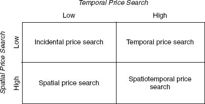
Consider a duopoly retail market for groceries in which price variations occur temporally (across weeks, because cycle time for price changes is weekly) within a store and spatially across stores. The duopoly assumption is reasonable and consistent with reality in many U.S. markets (Fox and Semple 2002), including the market we study.¹ Therefore, consumers can benefit from both temporal and spatial price search. For purposes of exposition, we split consumers into high and low types along the temporal and spatial price search dimensions. This leads to the four types of price search strategies among grocery shoppers (see Figure 1).

Grocery purchases through other retail formats have increased channel blurring (Inman, Shankar, and Ferraro 2004). We abstract away from this issue and focus only on the supermarket format.

Figure 1

Segmentation by Price Search Patterns

In the first segment, some shoppers do not search actively either across stores or across time, but they can still get low prices on promoted products because these products happened to be available on sale at their preferred store when they wanted to purchase them. We label this search strategy as “incidental price search.”

A second segment of shoppers tends to be mostly loyal to a preferred store and therefore does not take advantage of price variations across stores. This segment shifts purchases over time to take advantage of promotions at the preferred store. We label this search strategy as “temporal price search.”

A third segment of shoppers takes trips across stores to pick the best contemporaneous prices (on any given shopping trip) mostly to take advantage of cross-store spatial price differences. This type of shopper is the focus of Fox and Hoch's (2005) cherry-picking study. These shoppers may have less store loyalty than the previous two segments, though it is possible that they could buy most of their (non-deal) purchases at a preferred store and buy only low-priced items at other competing stores. We label this search strategy as “spatial price search.”

The fourth segment of shoppers takes advantage of both spatial and temporal price variations by making regular weekly shopping trips to both stores. These shoppers actively switch between the two stores and shift their purchase timing to get the best price deals across stores and over time for a grocery item. We label this search strategy as “spatiotemporal price search.”

Predictors of a Household's Price Search Strategy

We use a cost–benefit framework on the premise that consumers choose the search strategy that maximizes potential savings for their household, net of their costs (e.g., Putrevu and Ratchford 1997; Urbany, Dickson, and Kalapurakal 1996). Let W be the unit opportunity cost of travel time and T be the travel time to perform search. The travel time to perform search may be further decomposed into T = D/S, where D is the distance traveled to perform search and S is the speed of the typical mode of transport for grocery shopping. Then, the cost of search (C) is given by C = WT = W(D/S). In the context of grocery shopping in suburban markets in the United States, S can be assumed to vary little across consumers as a result of widespread car ownership in these markets. Thus, we focus on two variables: (1) D, the distance traveled to perform search, and (2) W, the unit opportunity cost of the household's time. We also consider certain stated personality characteristics and attitudes that may affect search behavior.

Geography

We denote a consumer's geographic location and the distances between the two closest competing stores for the consumer using the three-dimensional vector (D₁₂, D₁, D₂), where D₁₂ is the distance between the two stores, D₁ is the distance between the consumer's home and Store 1, and D₂ is the distance between the consumer's home and Store 2. To facilitate exposition, we treat distance as a dichotomous variable—large (L) or small (S)—though we consider both a dichotomous and a continuous variable specification for distance in our empirical analysis. We represent the relevant distances using a three-dimensional vector D₁₂D₁D₂; that is, if there is a segment with D₁₂ = L, D₁ = S, D₂ = L, we refer to that segment as LSL segment. We now explain our rationale behind how the spatial configurations of household and stores affect the household's choice of price search patterns. The pictorial descriptions in Table 1 under the column “Most Likely Consumer–Store Spatial Pattern” can be helpful in understanding the logic of our expectations.

Table 1

Summary of Expected Relationships and Empirical Results

Our expectation about the effect of spatial configuration on search behavior is based on the following basic argument: When stores are close to each other (i.e., D₁₂ = S), consumers will engage in greater spatial search; conversely, when stores are far away from each other (i.e., D₁₂ = L), consumers will engage in limited spatial search. Similarly, when the distance between a store and the consumer is small (i.e., when D₁ = S or when D₂ = S), the consumer will visit the corresponding store more often (i.e., he or she will engage in more temporal search at the store that is close to home); conversely, when D₁ = L or when D₂ = L, the consumer will visit the corresponding store less frequently (i.e., he or she will engage in less temporal search at the store that is far away from the home). Given these expectations, we now make specific predictions about the type of search pattern that households with different types of store–household spatial configurations will adopt.

Households of the type LLL, which are far away from either store and also face large interstore distances, are not likely to search much either spatially or temporally and therefore are most likely to adopt incidental price search.

Households of the types LSL or LLS, which are close to one of the stores, are likely to be loyal to the closer store (this would be their primary store) and perform temporal price search at their closest store because they can visit it more often. However, they do not perform much spatial price search because of the large interstore distance.

Households of the SLL type, which are located far away from either store, but both stores are close to each other, are most likely to use spatial price search. As we discussed previously, this is the behavior that Fox and Hoch (2005) focus on, and indeed they find that larger distances to the store and shorter interstore distances lead to greater cherry-picking behavior. Our study nests this prediction as part of a broader set of expectations. Finally, we expect that households of the SSS type are most likely to indulge in spatiotemporal price search to take advantage of both the spatial and the temporal price variation, given their close proximity to the stores and the small interstore distances.

We can also cross-validate the expectations about geography and price search by testing the price search effectiveness for the different geographic segments. Because the SSS segment searches both temporally and spatially, it should also have the greatest price search effectiveness. By the same logic, the LLL segment, which searches neither temporally nor spatially, should have the lowest price search effectiveness. The LSL and SLL segments should have intermediate levels of price search effectiveness.

Personal characteristics

Spatiotemporal price search requires the most effort and time, whereas incidental price search requires the least effort. Therefore, we expect that an increase in unit opportunity cost of time for a household reduces the likelihood of spatiotemporal price search the most and increases the likelihood of incidental price search the most. The net effect on the likelihood of a household choosing the two other intermediate price search patterns cannot be ordered but should lie between the two extreme patterns.

Some shoppers may have a greater ability to remember prices and organize information and thus have a lower cost to take advantage of market price variations through price search. Shoppers with greater price search skills who are more efficient in their price search are most likely to engage in spatiotemporal price search and least likely to engage in incidental price search.

Some consumers may derive utility from the price search process itself. For example, market mavens are shoppers who obtain “psychosocial” returns from sharing relevant market information with others rather than by the direct economic benefit to themselves. Thus, they collect relevant market information with the intent of sharing it with others (Feick and Price 1987; Urbany, Dickson, and Kalapurakal 1996). Urbany, Dickson, and Kalapurakal (1996) find that market mavens engage in more price search than others. We expect that this trait is least associated with incidental price search and most positively associated with spatiotemporal price search.

We summarize these expectations in Table 1 under the heading “Determinants of Price Search Patterns.” We also included several other demographic variables, such as age of head of household, sex of primary shopper, household size, and so on, in our empirical analysis, but these were not significant. To conserve space, we omit the discussion of the expectations associated with these other variables.

Effectiveness of the Different Price Search Strategies in Obtaining Low Prices

We adapt a construct that Ratchford and Srinivasan (1993) use to measure returns to price search for durable goods to quantify a household's observed price search effectiveness for grocery products. Intuitively, the effectiveness of a household's price search is the ratio of realized price savings to maximum potential savings, given the market price dispersions along both spatial and temporal dimensions. We propose the following measure of price search effectiveness for household i based on all the items purchased across multiple shopping trips n_i tracked over about one month:

\begin{matrix} {PSE}_{i} & = \frac{Actual savings captured for tracked trips}{Maximum potential savings for tracked trips} \\ = \frac{\sum_{j}^{n_{i}} {BV}_{ij}^{max} - \sum_{j}^{n_{i}} {BV}_{ij}^{*}}{\sum_{j}^{n_{i}} {BV}_{ij}^{max} - \sum_{j}^{n_{i}} {BV}_{ij}^{min}}, \end{matrix}

(1)

where $B V_{i j}^{\max} = Σ_{k = 1}^{m_{j}} Q_{i j k} P_{i j k}^{\max}$ is the maximum possible dollar value that household i could have paid for the shopping basket purchased on trip j, across stores and across time; $B V_{i j}^{\min} = Σ_{k = 1}^{n_{j}} Q_{i j k} P_{i j k}^{\min}$ is the minimum possible dollar value that household i could have paid for the shopping basket purchased on trip j, across stores and across time; and BV_ij^* is the actual dollar value that household i paid for the shopping basket purchased on trip j.

In this formulation, Q_ijk is the purchased quantity for item k, P_ijk^max is the maximum market price for item k across stores and time, and P_ijk^min is the minimum market price for item k across stores and time. Because BV_ij^max and BV_ij^min include both spatial and temporal market price dispersion for all the items in the shopping basket for trip j under consideration, we compute the maximum potential savings for each household “as if” it conducted a perfect spatiotemporal price search. This enables us to evaluate the effectiveness of all households on a comparable basis. If all the potential savings are captured, a household's price search effectiveness is 100%. Conversely, if every item was purchased at the highest price and no savings are captured by the household, the household's price search effectiveness is 0%.

If households' stated search patterns are consistent with observed behavior, households that claim to search more get lower prices on average. The self-declared “spatiotemporal” households should obtain the lowest prices on average (highest price search effectiveness), and the self-declared “incidental” price search households should pay the highest prices (lowest price search effectiveness) on average. The other two segments should pay the intermediate level of prices. It is of empirical interest as to whether “spatial” households or “temporal” households are more effective in obtaining better prices on average. We summarize these expectations in Table 1 under the column “Observed Price Search Effectiveness.”

Effect of Price Search Strategies on Retailer Profits

Our expectation is that profit margins will be greatest from households that search the least and lowest from those that search the most. Therefore, we expect that profit margins will be the greatest for the incidental cherry pickers and lowest for the spatiotemporal cherry pickers. For the other two segments, the profit margins will be intermediate. Whether the temporal cherry pickers have higher profit margins than the spatial cherry picker is an empirical question. We summarize these expectations in Table 1 under the column “Profit Margin.”

Although we state specific expectations about the relative levels of profit margins for the different search strategies, we do not have specific expectations about the average profits from households with the different search patterns. We expect that either the incidental cherry pickers (highest margins) or the temporal cherry pickers (highest loyalty and, therefore, greatest wallet share) will be the most profitable in terms of aggregate profits. However, the specific ordering of these two segments is an empirical question.

Data

Data Collection Strategy

The data are from four suburban areas of a midsize city in the northeastern United States in 2003–2004. Each area is effectively a duopoly with two regional competing grocery chains accounting for more than 85% market share. We obtained the cooperation of one of the grocery chains, which provided us with live access to customer transactions data at its stores on a daily basis. We label this cooperating chain as “Chain A” and the other chain as “Chain B.”

We selected a group of four stores of Chain A, paying special attention to the relative geographic distance between each of the stores and the corresponding nearest stores from Chain B. Specifically, we chose two Chain A stores that had competing Chain B stores within half a mile and another two Chain A stores that had competing Chain B stores more than two miles away. This ensured that there was significant variation in interstore distances in the data to test our expectations, and the distances are reasonably consistent with the average interstore distance of 1.43 miles and standard deviation for this suburban market. We also had geocoding information for all the loyalty card customers of Chain A, which we used to compute consumer–store distances.

As we stated previously, we augmented the transactional data of consumers obtained from Chain A to help answer our research questions in two ways: (1) We surveyed these consumers about their search behavior and other relevant attitudes toward grocery shopping, and (2) we collected the corresponding prices for the products purchased in Chain A in any given week at Chain B through direct observation by visiting Chain B.

We began with a survey of a random sample of customers on their visits to the four selected Chain A stores over three months during September 2003–November 2003. We staggered the surveys over three months because of constraints on the number of available interviewers.

The interviewers met shoppers at random while they were leaving the selected Chain A stores after their shopping trips and used “filter” questions to determine whether they qualified for inclusion in the sample for our study. The qualifying criteria were that (1) the intercepted shopper needed to be the primary grocery shopper for his or her household and (2) the shopper should have a “loyalty” card from Chain A. The second criterion ensured that we had identifier information (loyalty card number) to scan the transaction database of Chain A for shopping visits by the respondent. Because more than 95% of shoppers had a loyalty card, this was not very restrictive. If the intercepted shoppers met the qualifying criteria, the interviewer collected the following information about them: loyalty card number, which store they considered their primary store, and relative expenditure levels at the two competing chains. The interviewers then gave the qualified shoppers a detailed survey questionnaire containing relevant behavioral, attitudinal, and demographic questions with a request to return the finished questionnaire in a prepaid return envelope. If the responses were not returned within one month, we sent a reminder. We obtained responses from 255 shoppers, at a response rate of slightly less than 50%.

After we received the completed mail-in survey from a shopper, we used the identifier information (loyalty card number) to scan the transaction database of Chain A for shopping visits by this respondent on a daily basis. After we detected a shopping trip by this respondent, we obtained the prices for all the items in the shopping basket of the respondent over that week and the two following weeks at Chain A from the transaction database of Chain A. We obtained the contemporaneous price data from Chain B for all products in that household's basket by visiting the competing Chain B store for that week and the following two weeks.² This systematic (and labor-intensive) data collection approach ensured that we collected complete information on actual prices paid by a consumer as well as the temporal (over three weeks) and spatial (across the two competing retail chains) price variations for all the items purchased on any particular shopping trip.

We restricted data collection to baskets of only approximately ten households in any given week to make the manual data collection practical. Even with these households added, we needed to collect 600–700 prices in any given week because we also needed to collect intertemporal price data for households that we began tracking in the previous two weeks. When we received more than ten survey responses in a given week, we delayed data collection related to baskets of the excess households until we had a “lean” capacity to perform the data collection.

For all mail-in survey respondents, we performed the same process of obtaining price information for purchased items in their baskets for multiple trips. For most households, we obtained information for 3 trips. For a few households, we obtained only data on 2 trips within the data collection period. Overall, we collected price data on approximately 8500 distinct items over 710 shopping trips for the 255 households that responded to our survey. Considering that each item needed to be tracked over three weeks at Chain B by direct observation, we collected more than 25,000 price observations manually during a period of approximately six months in 2003 and 2004. Note that if a household did not use a loyalty card, it would not be found in our data. Approximately 87%–90% of the all commodity volume in the selected four stores in Chain A is accounted for by loyalty cards. However, because a household may not use a loyalty card when it does not avail of price promotions, our data may marginally overestimate price search effectiveness and underestimate retailer profit margins.

Finally, to address the question of the impact of price search on the retailer's profits, we obtained information about profits and profit margins of the 255 sample households with respect to Chain A over the 52 weeks of 2002. We also obtained profit and margin data for all loyalty card customers (21,963) from two of the sample stores of Chain A to conduct an in-depth investigation of customer profitability due to cherry-picking.

The Measures

We used self-reported consumer data to construct the various attitudinal and behavioral measures. The Appendix presents a complete list of the items used in each scale along with the corresponding scale reliability coefficients. When items were drawn from prior research, we note the specific sources. We developed the new measures in line with our conceptual framework and then modified them on the basis of personal interviews with a convenience sample of 14 grocery shoppers. We then used another convenience sample of 68 grocery shoppers to make initial assessments of reliabilities of all the multi-item scales used and to make any necessary adjustments in terms of dropping and modifying items.

We drew on the work of Feick and Price (1987) and Urbany, Dickson, and Kalapurakal (1996) to construct the “market mavenism” measure. The “perceived search skills” construct was based on the work of Putrevu and Ratchford (1997) and Urbany, Dickson, and Kalapurakal (1996). Whereas existing studies of consumers' stated price search propensities focus only on spatial price search, we distinguished between consumers' temporal and spatial price search propensities. We drew on existing research for the five items used in the spatial price search propensity scale. We developed the five items used in the temporal price search propensity scale.

We performed a two-segment cluster analysis (using Ward's method with squared Euclidean distances) of consumers' stated temporal and spatial price search propensity measures to classify consumers into high and low types along each dimension. The average scores on the temporal price search propensity for the high and low segments were 3.6 (SE = .039) and 2.1 (SE = .054) on a five-point scale. The large difference and the low standard errors indicate a high degree of discrimination between the high and the low types on the temporal dimension. The corresponding scores for the spatial price search propensity were 4.01 (SE = .038) and 2.32 (SE = .064), indicating a high degree of discrimination between the high and the low types on the spatial dimension as well. We also tested for the robustness of our results using a median split of consumers along the temporal and spatial dimensions based on the sum of the corresponding price search propensity scale items. The results are similar with such a split.

We computed the observed price search effectiveness of each household across multiple shopping trips (two to three trips) at Chain A, accounting for both the cross-store (across Chain A and Chain B) and intertemporal (over three weeks since the week of purchase) price dispersion in the market for all the items purchased in a trip. Because these tracked trips for each household are typically spread over one month, we can interpret the measure as the observed price search effectiveness of the household over a basket of monthly purchases at Chain A.

As Putrevu and Ratchford (1997) point out in their study, it is difficult to develop a multi-item scale for the unit opportunity cost measure that exhibits high scale reliability. At the same time, using the respondent's actual wage rate as a measure requires us to impute a wage rate for those who do not work. We follow Marmorstein, Grewal, and Fishe (1992) and Putrevu and Ratchford (1997) and use a single-item measure that asked respondents the hourly wage rate at which they would be willing to undertake an extra hour of work suitable to their skills.

We represent spatial pattern with three variables: distance of household to the closest Chain A store (D₁) and Chain B store (D₂) and distance between the two stores (D₁₂). Shopping trips involve fixed costs of travel to the stores and the actual time cost of shopping. With short distances, the time for shopping dominates travel time; thus, store–household distance may have limited impact on household decisions to make a trip. As the household–store distance increases, households may decide to reduce trips and consolidate their purchases. Thus, we expect that the effect of distance on the number of trips taken has threshold effects. Therefore, a binary categorization of distances seemed conceptually appropriate. We use the research design–driven natural break to classify stores close to each other (D₁₂ < .3 miles) as “small” and stores far away from each other (D₁₂ > 2 miles) as “large.” For distance between the household and the store, we report the results using a median split (1.8 miles) to classify distances as large or small. Our results are robust to changes in the split threshold over a wide range (1.4–2.2 miles) around the median value. We also test for whether threshold effects exist by directly including distance variables in the regression.

Results

Predictors of a Household's Price Search Strategy

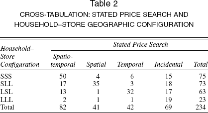
We first report a cross-tabulation of stated price search patterns against the geographic configuration of the household and stores in Table 2. For spatiotemporal, spatial, and temporal price search, the diagonal elements of the table have the highest frequency corresponding to each column, suggesting support for our expectations of the role of geography described previously. For example, the SSS configuration is most common among spatiotemporal price search households, the SLL configuration is most common among spatial price search households, and the LSL configuration is most common among temporal price search households. The incidental price search households are evenly distributed across the different types of location configurations, suggesting that opportunity cost should have an additional role other than geography in explaining the price search patterns. However, LLL households almost always choose incidental price search, consistent with our expectations.

Table 2

Cross-Tabulation: Stated Price Search and Household–Store Geographic Configuration

Household-Store Configuration	Stated Price Search
Household-Store Configuration	Spatiotemporal	Spatial	Temporal	Incidental	Total
SSS	50	4	6	15	75
SLL	17	35	3	18	73
LSL	13	1	32	17	63
LLL	2	1	1	19	23
Total	82	41	42	69	234

The results of the multinomial logit regression model appear in Table 3. The main explanatory variables are the cost of search variables: (1) the location configuration of the households and stores and (2) unit opportunity costs.

Table 3

Multinomial Logit Regression: Determinants of Price Search Patterns (Incidental Price Search and SSS is Base Case)

	Spatial Estimate (SE)	Temporal Estimate (SE)	Spatiotemporal Estimate (SE)
Intercept	–9.25^*** (2.35)	–3.16^** (1.51)	–3.05^* (1.77)
SLL	2.07^** (.81)	–.19 (.77)	–.48 (.73)
LSL/LLS	–2.51^* (1.29)	.62 (.62)	–1.97^*** (.70)
LLL	–12.01 (15.68)	–2.93^*** (.84)	–5.52^*** (.97)
Opportunity cost	–.08^*** (.03)	–.10^*** (.02)	–.24^*** (.03)
Market mavenism	1.07^*** (.33)	.54^** (.28)	.71^** (.29)
Perceived search skills	2.11^*** (.58)	1.19^*** (.45)	2.08^*** (.51)

p < .1.

p < .05.

***

p < .01.

Notes: We also included various demographic variables (age, sex, income, and household size) in the regression, but none of them were significant and therefore are not included here in the regressions we report.

We also use individual-specific variables, such as perceived search skills, and shopping-related personality traits, such as the self-perception of being a market maven.

The multinomial logit regression results appear in three columns in Table 3, one for each price search pattern (i.e., each variable of interest has different effects on the likelihood that a certain price search pattern is chosen). We have only three columns because we treat incidental price search as the base case, and the coefficients are relative to this base case. For the spatial configuration variables, we treat SSS as the base case.

The data support our expectations about the role of location configuration on price search patterns. We interpret the spatial configuration estimates across columns. The coefficient of SLL is highest (2.07) for spatial price search, as we expected; that is, when households are far away from both stores but the stores themselves are close to each other, the households are more likely to engage in spatial price search. The coefficient for LSL/LLS is significantly negative for spatial and spatiotemporal price search, suggesting that when stores are far apart, households are less likely to search spatially. However, the positive coefficient (correct sign) for temporal search is not significantly different from the base “incidental” price search case. The coefficient of LLL is significantly negative for spatial, temporal, and spatiotemporal price search, as we expected, suggesting that incidental price search is the most likely search pattern for the LLL household. Because SSS is treated as the base case in Table 3, we are unable to check whether SSS households prefer spatiotemporal cherry-picking. Therefore, we estimated the model with LLL as the base case. Indeed, SSS has significantly positive coefficients for the three price search patterns compared with the base case of incidental price search, in support of our expectation.³

A challenge with using LLL as the base case in the regression is that almost all LLL households engage in incidental price search; therefore, the predictor matrix becomes close to a singular matrix, leading to high standard errors on some of the coefficients.

As we expected, opportunity cost is significant and negative for all price search patterns, suggesting that an increase in opportunity cost decreases the likelihood of all three types of price search compared with incidental price search. An increase in opportunity cost has the greatest impact in reducing the likelihood of households using spatiotemporal price search (–.24) compared with incidental price search. The marginal effect of opportunity cost on temporal price search (–.10) and spatial price search (–.08) is not significantly different, though we expected the effect to be greater for spatial price search because that requires an additional trip to a competing store at the same time.

The effect of perceived search skills on the price search pattern is as we expected. People who perceive themselves as more skillful tend to engage in more spatial (2.11) and spatiotemporal (2.08) price search than temporal (1.19) or incidental (base case) price search. Perhaps the perceived search skill measure is more correlated with how well they can search for relevant price information across stores than within stores over time. As we expected, shopping mavens have a positive coefficient for spatial, temporal, and spatiotemporal search, consistent with their need to be key informants to others about the best prices available in the market.

The U² for the model in Table 3 is .45. With the location variables removed, the U² drops to .33. With location and opportunity cost removed, the U² with the perceived price search skills and mavenism drops to .09. Thus, although attitudinal variables help explain stated price search patterns, location and opportunity costs are the most important variables in explaining observed price search effectiveness and promotional responsiveness. This is particularly useful for retailers because they can implement targeted promotions using household geographic location and opportunity cost, information that is readily available to retailers from syndicated sources.

Effectiveness of the Different Price Search Strategies in Obtaining Low Prices

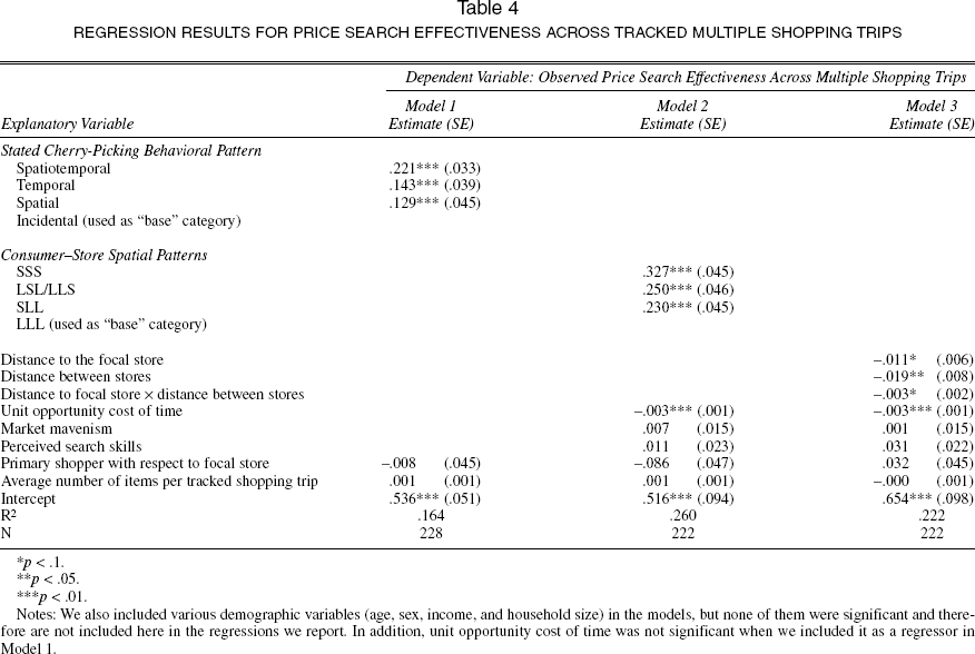
Next, we regress observed price search effectiveness against the stated price search patterns of households. We include the following controls: whether Chain A was the primary store and the average basket size (number of items) across tracked trips. The regression results appear in Model 1 of Table 4.

Table 4

Regression Results for Price Search Effectiveness Across Tracked Multiple Shopping Trips

Explanatory Variable	Dependent Variable: Observed Price Search Effectiveness Across Multiple Shopping Trips
Explanatory Variable	Model 1 Estimate (SE)	Model 2 Estimate (SE)	Model 3 Estimate (SE)
Stated Cherry-Picking Behavioral Pattern
Spatiotemporal	.221^*** (.033)
Temporal	.143^*** (.039)
Spatial	.129^*** (.045)
Incidental (used as “base” category)
Consumer–Store Spatial Patterns
SSS		.327^*** (.045)
LSL/LLS		.250^*** (.046)
SLL		.230^*** (.045)
LLL (used as “base” category)
Distance to the focal store			–.011^* (.006)
Distance between stores			–.019^** (.008)
Distance to focal store × distance between stores			–.003^* (.002)
Unit opportunity cost of time		–.003^*** (.001)	–.003^*** (.001)
Market mavenism		.007 (.015)	.001 (.015)
Perceived search skills		.011 (.023)	.031 (.022)
Primary shopper with respect to focal store	–.008 (.045)	–.086 (.047)	.032 (.045)
Average number of items per tracked shopping trip	.001 (.001)	.001 (.001)	–.000 (.001)
Intercept	.536^*** (.051)	.516^*** (.094)	.654^*** (.098)
R²	.164	.260	.222
N	228	222	222

p < .1.

p < .05.

***

p < .01.

Notes: We also included various demographic variables (age, sex, income, and household size) in the models, but none of them were significant and therefore are not included here in the regressions we report. In addition, unit opportunity cost of time was not significant when we included it as a regressor in Model 1.

As we expected, the incidental cherry picker has the lowest price search effectiveness but is still able to obtain 54% (the intercept) of the maximum potential savings. Notably, whereas the temporal cherry picker saves as much as 68% (intercept + temporal) of potential savings, the spatial cherry picker saves only 66% (intercept + spatial) of potential savings. However, households that engage in spatiotemporal cherry-picking are able to obtain as much as 76% (intercept + spatiotemporal) of the maximum potential savings.⁴ Thus, spatiotemporal cherry pickers have 22 percentage points greater price search effectiveness than incidental cherry pickers; the corresponding differences with respect to pure spatial cherry pickers and pure temporal cherry pickers are 14% and 13%, respectively.⁵

The coefficients for primary shopper and average number of items are not significant and do not have any impact on the savings percentage reported when they are omitted from the regression.

We used “prospective time windows” (i.e., purchase week + next two weeks) to account for temporal search in measuring relative price search effectiveness. Could the results differ with “prospective” and “retrospective” (i.e., purchase week +/– two weeks) time windows? We do not expect any systematic differences, because consumer inventory for the product during the survey week will be randomly distributed across both consumers and purchase categories. Because we cannot obtain “retrospective” field observations of competing prices at Chain B in the weeks before purchases at Chain A, we compare price search effectiveness within Chain A along only the temporal dimension with retrospective and prospective windows. The average price search effectiveness was virtually identical (.728 versus .726), and the correlation at the household level is .99.

Our results suggest that conscientious shoppers who shop at only one store but shift their purchase timing to take advantage of price specials at their loyal store can still obtain a significant fraction of the maximum potential savings. Those who also engage in spatial cherry-picking (i.e., spatiotemporal) increase their realized savings by an additional 8% of the maximum potential savings. Perhaps the most intriguing finding is that approximately 54% of the maximum possible savings are obtained by incidental search households that do not search for low prices at all. In other words, even a household that does not actively seek price promotion deals typically ends up capturing about half of the potential savings created by market promotions. Note that even if the household claims not to seek price promotions actively, it can purchase accelerate or stockpile when there is a promotion.

In Model 2, rather than using stated price search patterns as explanatory variables, we use the underlying “drivers”—location, opportunity cost, and attitudinal variables—that we identified previously (see Table 1) to explain price search effectiveness. The results are consistent with our expectations. We find that SSS households have the greatest price search effectiveness (with the highest estimated coefficient of .327) and that the LLL households have the lowest price search effectiveness (all estimated price coefficients are positive, when LLL is the base case).

Notably, we find that these underlying location variables have greater explanatory power than the stated price search patterns themselves.⁶ The R-square of the model increases from 16.4% to 26% when the underlying determinant variables of location pattern and available and relevant demographic variables (age, sex, income, and household size) are included. However, most of the explanatory power lies with the location and opportunity cost variables (24.9%), which together essentially capture the economic drivers of observed price search effectiveness. Of the 24.9% R-square, 17.7% comes from the location variables, and 7.2% comes from unit opportunity cost of time.⁷ This is an encouraging result because it suggests that geography and opportunity cost, information that is readily available to retailers, are the most useful predictors of how effective consumers are in taking advantage of price promotions. We further validate this by using these variables to predict consumers' stated price search patterns.

Becuase stated price search patterns already account for opportunity cost, it is not surprising that if opportunity cost is included in Model 1, it is not significant. Thus, we do not include opportunity cost in Model 1.

Households' incomes have a correlation of .75 with the opportunity cost measure. However, with household income as a proxy for opportunity cost, the explanatory power drops to approximately 4.6%, suggesting that the income measure is a noisier proxy for opportunity cost of time. The correlation of .75 suggests that wage rates are a reasonable proxy when stated opportunity cost data are unavailable. We thank a reviewer for suggesting this check.

Unfortunately, much of recent research on households' store choices using scanner data treats location and attitude/motivation variables as unobserved heterogeneity (e.g., Bucklin and Lattin 1992; Popkowski-Leszczyc, Sinha, and Timmermans 2000) and focuses on only pricing differences between stores at a single-category level (e.g., Bucklin and Lattin 1992). Therefore, it is not surprising that these studies are unable to explain store choice effectively. Thus, the omission of location information in empirical models of store choice (which treat locations as a source of unobserved heterogeneity) is a serious limitation. Our results also suggest that the extant theoretical research on retailer choice models that uses store and consumer locations and consumer opportunity costs within the Hotelling framework (e.g., Chan, Seetharaman, and Padmanabhan 2005; Thomadsen 2005) incorporates the empirically most important trade-offs in their models.

In Model 3, we report the results using distances directly in the model rather than as binary variables. As we expected, the distance between a household and its focal store and the distance between the focal and the competing stores have a negative impact, demonstrating that greater distances to the focal store and between the competing stores reduce the observed price search effectiveness of the household. Furthermore, consistent with the interaction effects identified in Model 2, we find a negative, significant interaction effect between the two distances. However, the R-square for the model drops from 26% to 22.2%. Thus, we conclude that Model 2, with discretized distances, has a greater explanatory power, providing evidence for threshold effects of distance in the decision to go shopping.

We do not find the average trip basket size to be significant in any of the three models. In retrospect, this is not surprising, because as basket values increase, the potential benefits increase; thus, although observed price search effectiveness does not change with basket size, the total savings obtained increases as basket size increases. We validate this argument in Table 3.

Here, we note a difference between our study and that of Fox and Hoch (2005). Fox and Hoch demonstrate that households shop across stores on a single day more often when they have larger baskets to purchase, but we do not test the endogeneity of trip size. First, we do not have data on whether consumers actually shopped at multiple stores on a single day to test this. Second, this is reasonable given our research focus on segmenting households on the basis of their overall price search behavior rather than segmenting the trips themselves. We measure average price search effectiveness of a household not over a given trip (as Fox and Hoch do) but rather over all trips in a given month.

Thus far, we have focused on the differences in observed price search effectiveness for the different price search patterns. Another issue pertains to the range of observed price variation in the market in the spatial dimension, temporal dimension, and spatiotemporal dimension. The average range of price variation has a natural interpretation. It can be interpreted as the “information value” of search along that dimension because this is the maximum potential savings that households can typically obtain by searching along that dimension (Baye, Morgan, and Scholten 2003). In Table 5, we report the information value (i.e., the average of maximum potential savings) along the spatial, temporal, and spatiotemporal dimensions based on the 710 tracked shopping baskets in our data. To gain insights into the role of basket size on potential benefits from search, we also report these values grouped by basket sizes. Note that we do not report information values for incidental price search, because any savings obtained is not from “active” search.

Table 5

“Information Value” from Price Search in Grocery Markets

Shopping Basket Value	Average Values of Maximum Potential Savings (SD)
Shopping Basket Value	Spatial	Temporal	Spatiotemporal
<$30	$2.98 (2.90)	$3.60 (5.90)	$5.04 (4.13)
$30-$60	$9.64 (5.79)	$11.47 (9.14)	$16.35 (9.29)
$61-$90	$16.41 (7.45)	$19.94 (9.87)	$27.36 (10.25)
>$90	$28.02 (11.56)	$31.02 (18.1)	$45.05 (19.34)
Sample average: $31.22	$7.20 (5.65)	$8.49 (6.45)	$11.99 (9.39)

As we expected, the information value is greater for larger baskets across the three different search patterns in which consumers can actively engage. The information value is convex in basket size; that is, savings from large baskets are more than proportionately greater than savings from small baskets. For basket values greater than $90, along the spatioemporal dimension, a household can potentially save $45 on average. For basket values of $60–$90, the average potential savings drop to approximately $27. The corresponding average is approximately $16 on basket values of $30–$60 and only approximately $5 on basket values less than $30.

Not surprisingly, the information value is greatest along the spatiotemporal dimension across all basket sizes ($11.99). Notably, the information value of $8.49 from price search on purely the temporal dimension is greater than $7.20 savings from search on purely the spatial dimension. Although we recognize that this result should be tested for generalizability across other retailers and in other competitive environments, it is a surprising empirical finding that potential for savings is greater from temporal search than for spatial search in this market.

Effect of Price Search Strategies on Retailer Profits

How do price search patterns affect retailer profits? We use data on actual shopping trips at Chain A by the 255 surveyed households over 52 weeks in 2002 to compute average profit margins and weekly profits to the store. By using data over the whole year (rather than during the study period), we obtain more robust measures of profits.

The top panel of Table 6 reports the averages for margins and weekly profits per household, broken down by stated price search patterns and by observed household–store spatial patterns. In addition, we report some descriptive statistics, such as trip frequency, basket sizes, and the self-reported wallet shares at Chain A.

Table 6

Averages of Retailer Performance Measures at the Cooperating Chain

Store Performance–Related Measures at the Cooperative Retail Chain	For All Shoppers	By Stated Price Search Pattern				By Observed Household–Store Spatial Configuration
	For All Shoppers	Spatiotemporal	Temporal	Spatial	Incidental	SSS	LSL	SLL	LLL
Surveyed Sample (N = 255)
Average profit margin^a,b	.23	.21	.22	.23	.26	.19	.24	.24	.33
Average trip frequency^a	.94	1.18	1.12	.74	.66	1.21	1.02	.77	.48
Wallet share^a,c	.61	.62	.67	.56	.60	.63	.70	.62	.53
Average trip basket size^a	$35.43	$25.30	$33.28	$30.65	$51.22	$25.78	$33.91	$35.38	$67.96
Average weekly profit^a,b	$7.20	$6.83	$8.67	$5.85	$7.47	$6.57	$8.78	$6.45	$9.06
All Households at Two of the Stores Included in Study (N = 21,963)
Average profit margin^a,b	.25					.21	.26	.25	.32
Average trip frequency^a	.72					1.04	.76	.60	.45
Average trip basket size^a	$33.34					$25.26	$30.73	$35.25	$44.34
Average weekly profit^a,b	$5.58					$5.21	$5.93	$5.42	$5.99

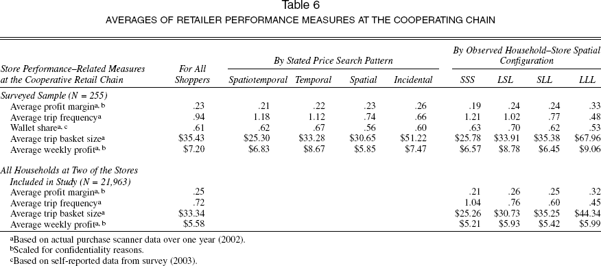
Based on actual purchase scanner data over one year (2002).

Scaled for confidentiality reasons.

Based on self-reported data from survey (2003).

The averages across different price search patterns are consistent with our expectations. For example, the average profit margin per household is the highest for the incidental cherry pickers and the lowest for the spatiotemporal cherry pickers, with a difference in profit margins of approximately 20%. Consistent with our estimates of price search effectiveness, we find that households that engage in temporal or spatial price search provide intermediate profit margins. Our results are also reassuring to retailers in the sense that even the most price search–intensive spatiotemporal segment brings a positive average contribution to the bottom line.

In terms of total weekly profits, the temporal segment provides the greatest average profits—even greater (by approximately 15%) than the incidental price search segment. Although the store-loyal temporal segment has lower margins than the incidental segment, its average wallet is 67%, compared with the 60% wallet share of households that engage in incidental price search. This explains why we found greater average profits from households in the temporal segment even though they have lower profit margins.

The averages in Table 6 are also consistent with our expectations for the household–store spatial patterns. For example, the profit margins are greatest for LLL households and lowest for SSS households. In contrast, SSS households visit the store most often, and LLL households visit least often. As we expected, LLL households had the largest baskets, and SSS households had the smallest baskets. Notably, the aggregate weekly profits are greatest for the LLL households and the LSL households. In other words, the greatest aggregate profits are obtained from households when the two competing stores are farther apart and cross-store shopping is least likely.⁸

After we account for the purchases at Chain A and the stated share of Chain A, the average weekly basket size is $62.48 (approximately $65 including taxes on nonfood items). This estimate is at the low end of published estimates of weekly household expenditures. This may be because the stated share of Chain A did not properly account for purchases of nonfood products through other channels, such as drugstores and warehouse clubs.

To check whether these differences in averages of margins and weekly profits across the different segments are statistically significant, we performed regressions with different store performance measures as dependent variables and the stated cherry-picking patterns/spatial pattern as explanatory variables. We also included additional control variables (e.g., household size). As reflected in our analysis of means in Table 6, the regression results show that the relative differences are not only consistent with our expectations but also statistically significant.

Extreme Cherry-Picking: Do Certain Households Provide Negative Net Margins?

Our analysis shows that, on average, all the price search segments are profitable. With the increased use of loss leaders in grocery retailing, a concern in the academic and trade literature (e.g., Dreze 1999; McWilliams 2004; Mogelonsky 1994) is that there are some “extreme” cherry pickers—dubbed the “devils” customer group—who mostly buy only loss-leader items, thus yielding negative gross margins for the retailer. If the proportion of such cherry-picking households is indeed large, loss-leader pricing to increase store traffic may be unprofitable, and strategies to discourage such households might be required (Dreze 1999; Levy and Weitz 2004). Therefore, we attempt to quantify the size of the extreme-cherry-picking segment and the extent of losses due to them.

For a robust analysis of extreme-cherry-picking households, we needed a larger sample than the 255 we used in the previous analysis. Therefore, we used a database with all loyalty-card holder households at two stores (one with the competitive store close and the other with the competitive store farther away; they are also two of the four stores used in our actual sample study) of Chain A for which we have their nine-digit zip code data. These 21,963 households account for more than 75% of total sales in 2002 in each of the stores. We also infer whether these households use Chain A as their primary grocery store.⁹ For comparison with our in-sample households, we report the same measures (except the self-reported wallet share measures) in the bottom panel of Table 6.

Chain A is classified as a primary (secondary) store for a household if the actual annual grocery spending of that household at Chain A in 2002 is at least 70% (less than 30%) of the average annual grocery spending for households in the same census block group as the given household. The census block group–level grocery spending data are available to Chain A from syndicated data services. The classification results using this criteria for our sample of 255 households have a correlation of .87 with those based on consumers' self-reports in our survey.

The larger sample is virtually identical to the surveyed sample in terms of relative magnitudes of average profit margins, trip frequency, and basket size for the different segments. For weekly profits, although the relative magnitudes across the groups are the same, the larger sample has lower total profits, especially for the LSL and the LLL households. This suggests that our surveyed sample systematically oversampled households that spent more at Chain A. However, because the profit margins are almost identical, there is little cause for bias in the price search effectiveness regressions we reported previously.

In terms of extreme cherry-picking, only 1.2% of the 21,963 households (i.e., 255 households) contribute a net negative profit to the store over the one-year period. As we expected, these are all secondary shoppers with respect to Chain A. The small number is also consistent in our sample of 255 households. Only 1.7% of in-sample households (i.e., 4 of 255) contributed a net negative margin during 2002; again, these 4 households were secondary shoppers with respect to Chain A.

What are the characteristics of extreme cherry pickers? Their average trip basket size is only $13.60 (versus $33.34 for all households). In addition, a trip-level analysis of these extreme cherry pickers indicates that approximately 27% (70) of the 255 households engaged in at least one “exclusive loss-leader trip” during 2002. We characterized an exclusive loss-leader trip as a shopping trip in which at least 90% of all the items purchased by the customer on that trip are loss-leader items and there are at least four such items in the basket. Finally, the spatial pattern distribution for these 255 households is consistent with our expectations. In terms of grouping the extreme-cherry-picking households by location patterns, the largest group belonged to the SSS location pattern (44%). This was followed by the SLL (38%) and LSL (18%) pattern.

What is the impact of this extreme group of cherry pickers (who are all secondary shoppers) on the chain's overall profits? The net loss from these households is approximately .2% of the total aggregate positive profit to Chain A from the rest of its customers, approximately .8% of profits from customers belonging to the SSS location pattern (the households most likely to engage in cross-store intertemporal shopping), and approximately 1.2% of profits from the all secondary shoppers. Therefore, we conclude that extreme cherry pickers have little impact on overall retailer profitability. This is in stark contrast to conventional wisdom that losses produced by these extreme cherry pickers (dubbed the “devils”) wipe out profits generated by the profitable customers (dubbed the “angels”) (McWilliams 2004). However, the generalizability of our findings needs to be assessed with future analyses across other market and product contexts.

Conclusion

This article introduces an integrated analysis of spatial and temporal price search in response to price promotions and its impact on retailer profitability. Extant research has treated the temporal and spatial dimensions separately and therefore has underestimated the impact of retail promotions on household response and retail profitability. Using a novel but labor-intensive data collection approach that combined observational and survey data, we assembled a data set amenable for such an integrated analysis. The key empirical insights from our analysis are as follows:

Price search patterns and price search effectiveness are largely driven by geography (store and consumer locations) and opportunity costs. Other individual-specific variables have limited impact. This suggests that a retailer can implement targeted promotions using price search as a segmentation variable because of the easy availability of geography and demographic data.

Pure temporal and spatial price search households roughly have the same levels of price search effectiveness. Consumers who claim not to search at all (“incidentals”) obtain approximately 50% of the potential savings by being at the right place at the right time. Even the segment that searches the most (the spatiotemporal segment) saves only approximately 75% of the potential savings in the marketplace.

The temporal search segment contributes most to the total profits of the retailer, even more than the incidental price searchers, who have greater profit margins. This suggests that periodic price promotions serve an important defensive role in retaining profitable store-loyal households (Little and Shapiro 1980).

Contrary to conventional wisdom that extreme cherry pickers have a significant, negative impact on retailer profits, we find that the impact of these households on retail profits is minimal.

Limitations and Suggestions for Further Research

Certain limitations in this study suggest some possibilities for further research. First, we focused on four sets of competitive stores within one suburban market. Further research should investigate markets with different characteristics to assess both the generalizability of our specific results and how these characteristics affect price search effectiveness. Specifically, stores tend to be clustered closer in urban/suburban markets, but they tend to be farther apart in rural markets. Thus, the proportion of people following different price strategies is likely to be different in such markets, though our inferences of price search effectiveness and retail profit margins for the different search strategies are likely to be more stable.

Second, we focused on price search effectiveness across the entire basket of purchases made by households. Although this is a useful step, a deeper investigation of how price search effectiveness varies across categories (e.g., stockpilable versus nonstockpilable, regularly versus irregularly purchased categories, impulse versus planned purchases) could provide marketing managers with additional insights. Examples of studies on category characteristics are Bell, Chiang, and Padmanabhan (1999) and Narasimhan, Neslin, and Sen (1996).

Third, it would be worthwhile to study how price search effectiveness can be affected by the use of marketing-mix variables, such as features and displays. Features may affect spatial efficiency more, whereas displays may affect temporal efficiency more. Overall, there is an opportunity to understand how price search effectiveness varies as a function of (1) market characteristics, (2) category characteristics, and (3) marketing-mix variables.

In this study, we investigated the spatial and temporal dimensions of cherry-picking. A third dimension in which consumers can choose to get lower prices for their groceries is through brand switching (the “brand” dimension). Accounting for this third dimension could mean that the opportunity for savings in the market could be greater. However, incorporating the brand dimension of price search in estimating price search effectiveness is difficult because it requires extensive purchase histories of consumers or subjective judgments by researchers to identify household-level “substitute brands and consideration sets” in each product category. Nevertheless, to gauge the robustness of our results, we compared price search effectiveness in branded categories with nonbranded product categories (e.g., fresh meat, seafood, fruits, vegetables, baked goods), in which the brand-switching dimension is irrelevant. As we expected, the estimated price search effectiveness is marginally higher for nonbranded product categories (.67 versus .64) because there is no downward bias from ignoring brand switching. However, the ordering of segments based on stated price search patterns and spatial locations is identical to the results reported. However, a systematic study of cherry-picking that includes the brand dimension along with the spatial and temporal dimensions should be a focus of further research.

One data limitation of our study is that we have data on purchases only from one chain. It is reasonable to question whether the absence of purchase data from the second chain might bias our estimates of price search effectiveness and retail profits. Fox and Hoch (2005) show that households selectively use secondary stores on cherry-picking trips to purchase promoted items disproportionately. In our data, approximately 20% of shoppers were secondary shoppers at Chain A. Consistent with Fox and Hoch, we find that, on average, secondary shoppers have higher price search effectiveness and lower profit margins (.68, .22) than primary shoppers (.67, .23). However, because our data from Chain A include both secondary and primary shoppers, our estimates are unlikely to be biased as long as secondary shoppers are correctly represented in our sample. Further research with larger sample sizes should systematically test for any differences in the temporal and spatial price search behavior of primary and secondary shoppers.

There is a long research tradition of inferring consumer preferences and sensitivity to prices and other marketing-mix variables using consumers' observed choice behavior. These analyses are typically for a single category. There has been a recent trend in studying choices across categories (e.g., Chib, Seetharaman, and Strijnev 2002; Manchanda, Ansari, and Gupta 1999). In terms of store choice, a few studies model consumer store choice with data from a single category (e.g., Bucklin and Lattin 1992). Bell and Lattin (1998) model consumer choice between everyday low prices and high/low store formats at the basket level rather than at the single-category level on the grounds that consumers make store choices based on the total cost of shopping for their entire basket. This analysis accounts for spatial cherry-picking but does not model temporal cherry-picking. A model incorporating temporal cherry-picking needs to extend the current literature on dynamic structural models of consumer choice (e.g., Sun, Neslin, and Srinivasan 2003), in terms of both estimation methodology and modeling.

The insights gained from our descriptive analysis of cherry-picking patterns across stores at the basket level should be insightful in developing a structural model of store competition that accounts for the notion that consumers choose stores on the basis of their baskets of purchases and can choose from either intertemporal or cross-store cherry-picking patterns. Furthermore, with the increasing variety of retail formats available (e.g., mass merchandisers, supermarkets, wholesale clubs) for grocery purchases, there has been an interest in how consumers choose across retail formats depending on their locations and needs (e.g., Fox, Montgomery, and Lodish 2004; Inman, Shankar, and Ferraro 2004). We hope that this article serves as an impetus for launching further research.

Footnotes

Appendix List of Items for Various Multi-Item Scale Constructs Used in the Empirical Analyses

All items were responses from mail surveys and were evaluated on a five-point scale anchored by “strongly agree” and “strongly disagree.”

Temporal Price Search Propensity (five items; Cronbach's α = .82)

•

I usually plan the timing of my shopping trip to a particular grocery store in such a way so as to get the best price deals offered at that store.^a

•

There are times when I delay my shopping trip to wait for a better price deal.^a

•

Although planned before making a shopping trip, I often do not buy some items if I think they will be on better deal shortly.^a

•

I keep track of price specials offered for the grocery products at the stores I regularly buy from.^a

•

To get the best price deals for my groceries I often buy the items I need over 2 or 3 trips.^a

Spatial Price Search Propensity (five items; Cronbach's α = .89)

•

I often compare the prices of two or more grocery stores.^b

•

I decide each week where to shop for my groceries based upon store ads/fliers.^b

•

I regularly shop the price specials at one store and then the price specials at another store.^b

•

Before going grocery shopping I check the newspaper for advertisements by various supermarkets.^c

•

To get the best price deals for my groceries I often shop at 2 or 3 different stores.^c

Market Mavenism (four items; Cronbach's α = .89)

•

I like it when people ask me for information about products, places to shop, or sales.^b,d

•

I like it when someone asks me where to get the best buy on several types of products.^b,d

•

I know a lot of different products, stores, and sales and I like sharing this information.^b,d

•

I think of myself as a good source of information for other people when it comes to new products or sales.^b,d

Perceived Search Skills (eight items; Cronbach's α = .71)

•

I know what products I am going to buy before going to the supermarket.^c

•

I am a well-organized grocery shopper.^c

•

Before going to the supermarket, I plan my purchases based on the specials available that week.^c

•

I can easily tell if a sale/special price is a good deal.^c

•

It is very difficult to compare the prices of grocery stores (reverse coded).^b

•

It is very difficult to compare the quality of meat and produce between grocery stores (reverse coded).^b

•

I prepare a shopping list before going grocery shopping.^c

•

I presort my coupons before going grocery shopping.^c

New item developed in this study.

Urbany, Dickson, and Kalapurakal (1996).

Putrevu and Ratchford (1997).

Feick and Price (1987).

References

ACNielsen (2006), “Promoted Volume: Are You Driving Purchases or Renting Consumers?” paper presented at the Consumer360 Conference, (May 16), (accessed June 2006), [available at http://www.consumer360.com/sessions.html].

Kearney

A.T.

(2005), “Sidebar: Best Practices in Pricing and Promotion,” (accessed December 16, 2005), [available at http://www.atkearney.com/main.taf?p=5,3,1,113#8].

Baye

Michael R.

, Morgan

John

, and Scholten

Patrick

(2003), “The Value of Information in an Online Consumer Electronics Market,” Journal of Public Policy & Marketing, 22(Spring), 17–25.

Beatty

Sharon E.

, and Smith

Scott M.

(1987), “External Search Effort: An Investigation Across Several Product Categories,” Journal of Consumer Research, 14(June), 83–95.

Bell

David R.

, Chiang

Jeongwen

, and Padmanabhan

(1999), “The Decomposition of Promotional Response: An Empirical Generalization,” Marketing Science, 18(4), 504–526.

Bell

David R.

, Chiang

Jeongwen

, and Lattin

James M.

(1998), “Shopping Behavior and Consumer Preference for Store Price Format: Why ‘Large Basket’ Shoppers Prefer EDLP,” Marketing Science, 17(1), 66–88.

Bucklin

Randolph E.

, and Lattin

James M.

(1992), “A Model of Product Category Competition Among Grocery Retailers,” Journal of Retailing, 68(3), 271–93.

Carlson

John A.

, and Gieseke

Robert J.

(1983), “Price Search in a Product Market,” Journal of Consumer Research, 9(March), 357–65.

Chan

Tat Y.

, Seetharaman

P.B.

, and Padmanabhan

(2005), “Modeling Locations and Pricing Decisions in the Gasoline Market: A Structural Approach,” working paper, Olin School of Business, Washington University, St. Louis.

10.

Chib

Siddhartha

, Seetharaman

P.B.

, and Strijnev

Andrei

(2002), “Analysis of Multi-Category Purchase Incidence Decisions Using IRI Market Basket Data,” Advances in Econometrics, 16, 57–92.

11.

Conlisk

John

, Gerstner

Eitan

, and Sobel

Joel

(1984), “Cyclic Pricing by a Durable Goods Monopolist,” Quarterly Journal of Economics, 99(3), 489–505.

12.

Cooper

Lee G.

, and Nakanishi

Masao

(1988), Market Share Analysis: Evaluating Competitive Marketing Effectiveness. Boston: Kluwer Academic.

13.

Dreze

Xavier

(1999), “Rehabilitating Cherry Picking,” working paper, Marshall School of Business, University of Southern California.

14.

Feick

Linda F.

, and Price

Lawrence L.

(1987), “The Market Maven: A Diffuser of Marketplace Information,” Journal of Marketing, 51(January), 83–97.

15.

Fox

Edward J.

, and Hoch

Stephen J.

(2005), “Cherry-Picking,” Journal of Marketing, 69(January), 46–62.

16.

Fox

Edward J.

, Montgomery

Alan L.

, and Lodish

Leonard M.

(2004), “Consumer Shopping and Spending Across Retail Formats,” Journal of Business, 77(2), S25–S60.

17.

Fox

Edward J.

, Montgomery

Alan L.

, and Semple

John

(2002), “Understanding Cherry-Pickers: How Retail Customers Split Their Shopping Baskets,” working paper, Cox School of Business, Southern Methodist University.

18.

Hoch

Stephen J.

, Kim

Byung-Do

, Montgomery

Alan

, and Rossi

Peter E.

(1995), “Determinants of Store-Level Price Elasticity,” Journal of Marketing Research, 32(February), 17–29.

19.

Huff

L. David

(1964), “Defining and Estimating a Trading Area,” Journal of Marketing, 28(July), 34–38.

20.

Inman

J. Jeffrey

, Shankar

Venkatesh

, and Ferraro

Rosellina

(2004), “The Roles of Channel-Category Associations and Geodemographics in Channel Patronage,” Journal of Marketing, 68(April), 51–71.

21.

Jacobson

Robert

, and Obermiller

Carl

(1990), “The Formation of Expected Future Price: A Reference Price for Forward-Looking Consumers,” Journal of Consumer Research, 16(4), 420–32.

22.

Levy

Michael

, and Weitz

Bart A.

(2004), Retailing Management. New York: McGraw-Hill/Richard D. Irwin.

23.

Little

John D.C.

, and Shapiro

Jeremy F.

(1980), “Theory for Pricing Nonfeatured Products in Supermarkets,” Journal of Business, 53(3), 199–209.

24.

Mace

Sandrine

, and Neslin

Scott A.

(2004), “The Determinants of Pre- and Postpromotion Dips in Sales of Frequently Purchased Goods,” Journal of Marketing Research, 41(August), 339–50.

25.

Manchanda

Puneet

, Ansari

Asim

, and Gupta

Sunil

(1999), “The ‘Shopping Basket’: A Model for Multicategory Purchase Incidence Decisions,” Marketing Science, 18(2), 95–114.

26.

Marmorstein

Howard

, Grewal

Dhruv

, and Fishe

Raymond P.H.

(1992), “The Value of Time Spent in Price Comparison Shopping: Survey and Experimental Evidence,” Journal of Consumer Research, 19(June), 52–61.

27.

McWilliams

Gary

(2004), “Minding the Store: Analyzing Customers, Best Buy Decides Not All Are Welcome,” The Wall Street Journal (Eastern edition), (November 8), A1.

28.

Mela

Carl F.

, Jedidi

Kamel

, and Bowman

Douglas

(1998), “The Long-Term Impact of Promotions on Consumer Stockpiling,” Journal of Marketing Research, 35(May), 250–62.

29.

Mogelonsky

Marcia

(1994), “Please Don't Pick the Cherries,” Marketing Tools, (September–October), 10.

30.

Narasimhan

Chakravarthi

, Neslin

Scott A.

, and Sen

Subrata K.

(1996), “Promotional Elasticities and Category Characteristics,” Journal of Marketing, 60(April), 17–30.

31.

Neslin

Scott A.

, Henderson

Caroline

, and Quelch

John

(1985), “Consumer Promotions and the Acceleration of Product Purchases,” Marketing Science, 4(2), 147–65.

32.

Newman

W. Joseph

(1977), “Consumer External Search: Amount and Determinants,” in Consumer and Industrial Buying Behavior, Woodside

Arch

, Sheth

Jagdish

, and Bennett

Peter

, eds. New York: Elsevier, 79–84.

33.

Popkowski-Leszczyc

Peter T.L.

, Sinha

Ashish

, and Timmermans

Harry J.P.

(2000), “Consumer Store Choice Dynamics: An Analysis of the Competitive Market Structure for Grocery Stores,” Journal of Retailing, 76(3), 323–44.

34.

Putrevu

Sanjay

, and Ratchford

Brian T.

(1997), “A Model of Search Behavior with an Application to Grocery Shopping,” Journal of Retailing, 73(4), 463–86.

35.

Ratchford

Brian T.

, and Srinivasan

Narasimhan

(1993), “An Empirical Investigation of Returns to Search,” Marketing Science, 12(1), 73–87.

36.

Sobel

Joel

(1984), “The Timing of Sales,” Review of Economic Studies, 51(3), 353–68.

37.

Sun

Baohong

, Neslin

Scott A.

, and Srinivasan

Kannan

(2003), “Measuring the Impact of Promotions on Brand Switching When Consumers Are Forward Looking,” Journal of Marketing Research, 40(November), 389–405.

38.

Thomadsen

Raphael

(2005), “The Effect of Ownership Structure on Prices in Geographically Differentiated Industries,” Rand Journal of Economics, 36(4), 908–929.

39.

Urbany

Joel E.

, Dickson

Peter E.

, and Kalapurakal

Rosemary

(1996), “Price Search in the Retail Grocery Market,” Journal of Marketing, 60(April), 91–104.

40.

Urbany

Joel E.

, Dickson

Peter E.

, and Sawyer

Alan G.

(2000), “Insights into Cross- and Within-Store Price Search: Retailer Estimates vs. Consumer Self-Reports,” Journal of Retailing, 76(2), 243–58.

41.

Varian

Hal R.

(1980), “A Model of Sales,” American Economic Review, 70(4), 651–59.