Determining Consumers’ Discount Rates with Field Studies

Abstract

Because utility/profits, state transitions, and discount rates are confounded in dynamic models, discount rates are typically fixed for the purpose of identification. The authors propose a strategy of identifying discount rates. The identification rests on imputing the utility/profits using decisions made in a context in which the future is inconsequential, the objective function is concave, and the decision space is continuous. They then use these utilities/profits to identify discount rates in contexts in which dynamics become material. The authors exemplify this strategy using a field study in which cell phone users transitioned from a linear to a three-part-tariff pricing plan. They find that the estimated discount rate corresponds to a weekly discount factor (.90), lower than the value typically assumed in empirical research (.995). When using a standard .995 discount factor, they find that the price coefficient is underestimated by 16%. Moreover, the predicted intertemporal substitution pattern and demand elasticities are biased, leading to a 29% deterioration in model fit and suboptimal pricing recommendations that would lower potential revenue gains by 76%.

Keywords

dynamic structural model identification forward-looking consumers pricing three-part tariff discount rate

Consumers often face situations in which they must choose either to engage in consumption in the present or wait to consume in the future. A rich stream of recent literature has adopted dynamic structural models to study intertemporal consumption, yielding deep insights into consumer behavior (see, e.g., Erdem and Keane 1996; Hendel and Nevo 2006; Rust 1987; Sun 2005). Although the use of structural models to study dynamic consumption behavior is increasingly ubiquitous, the identification of these models is problematic (Rust 1994). To identify consumer utility functions, it is often necessary to assume or fix the discount factor at a given value. In contrast, we develop a dynamic structural model to identify and measure consumer discount rates using field data. The identification strategy relies on the intuition that we can impute consumers’ utility when their current decisions are inconsequential for their future decisions, the objective function is concave, and the decision space is continuous. Then, conditioned on the estimated utilities under this static setting, it becomes possible to identify discount rates when future outcomes become material to these consumers’ decisions. We outline a proof of identification and use a Monte Carlo simulation to show the sampling properties of the identification approach.

The identification strategy has general applications in contexts in which researchers have repeated observations of firms or consumers making continuous decisions under both static and dynamic settings. These include observations of consumers’ reward points usage decisions in loyalty programs with expiration dates, usage consumption decisions for Internet or cell phone data access plans with a monthly fixed allowance that does not roll over, firms’ markdown pricing for end-of-season clearance inventory, and sellers’ pricing decisions on perishable goods such as ticket sales. In auctions, for example, consumers may face posted prices for some goods and auctions for others. When consumers face identical items that are auctioned off sequentially, the intertemporal trade-off is consequential and affects the bidding behavior (e.g., Zeithammer 2006). The posted price context in which consumers make static decisions can then be used to infer preferences. Likewise, in the context of firms’ markdown pricing of seasonal goods such as swimwear and skis for which styles change each year, intertemporal substitution between the final markdown period and the future is minimized in that period; thus, the pricing decision in final periods becomes static and can be used to infer firms’ objective functions. What these contexts have in common is that there are multiple observations of decision making in periods that are independent of dynamics. The repeated observations of static data provide information needed for identifying the preferences, which can then be used in the dynamic contexts to infer discount rates.

To exemplify this approach, we apply it to consumer cell phone minute usage data during a field study that involves switching consumer pricing plans. In our data, consumers were initially under a linear “pay-per-minute” plan; thus, usage decisions involved no intertemporal tradeoffs because usage early in the month had no bearing on prices paid later in the month. Subsequently, the cell phone service provider switched consumers to a nonlinear three-part tariff plan.¹ The plan switch induced intertemporal substitution trade-offs as consumers’ minute usage decisions early in the month had consequences for the rates they faced later in the month. The results indicate that consumers have weekly discount factors in our data of approximately .9 with a 95% confidence interval of (.78, .97).² The .995 discount factor, which is typically assumed in the literature, implies that a consumer would accept 1 minute and 1 second at the end of the month as a substitute for an equally priced minute at the beginning of the month. In contrast, we compute that consumers value a minute more closely to 1 minute and 30 seconds at the end of the month.

A three-part tariff plan contains three components: an access fee, a certain amount of allowance minutes, and a marginal price if the consumer's usage exceeds the allowance within a billing cycle. As a result, the consumer may be subject to extra fees when the consumption exceeds the allowance (overage) and overpays if the consumption falls below the allowance (underage). Because of the allowance and the high marginal price, a consumer must decide how to allocate his or her consumption across time within a billing cycle, intending to avoid overage and underage so as to maximize total utility.

The implied weekly discount rates are approximately 1.11 with a 95% confidence interval of (1.03, 1.28).

We organize the remainder of the article as follows: Next, we provide an overview of the relevant literature to differentiate the current study from previous research. Then, we detail our identification strategy, and to exemplify our identification strategy, we detail our modeling context. Next, we report a Monte Carlo simulation to demonstrate the validity of the identification strategy and then apply the approach to a field setting. Subsequently, we present and discuss the results and sensitivity analyses. We conclude with some managerial implications and future research directions.

Relevant Literature

Given that discount rates are not typically identified, several approaches have emerged to contend with the problem, including (1) assuming a fixed value for the discount rate, (2) functional identification using structural assumptions and/or estimation using exclusion restrictions, and (3) experimental approaches. Table 1 provides an overview of a sample of these approaches and their resulting discount values converted to their weekly equivalents. Table 1 makes it apparent that discount rates vary considerably across studies: The mean weekly discount factor is .98 with a standard deviation of .032. The corresponding weekly discount rates average 2.09% with a large standard deviation of 3.66%. In short, there is no clear consensus regarding the value of discount factors, partially because discount rates are typically not identified.

Table 1

Example Discount Rates In Empirical Studies

Study	Choice Domain	Approach^a	Discount Factor	Period	Weekly Discount Factor	Implied Weekly Interest Rate (%)
Rust (1987)	Bus engine replacement	F	.9999	Month	→ 1	.002
Hotz and Miller (1993)	Children/sterilization	E	.65 (.68)	Year	.992	.83
Erdem and Keane (1996)	Laundry detergent	F	.995	Week	.995	.50
Ackerberg (2003)	Yogurt	E	.98 (.02)	Week	.98	2.04
Hartmann (2006)	Golf	F	.99	Day	.932	7.29
Gordon (2009)	Personal computers	F	.98	Month	.995	.47
Kim, Albuquerque, and Bronnenberg (2010)	Camcorders	F	1.0	Minutes	1.0	0
Goettler and Clay (2011)	Online grocery service	E	.974 (.001)	Week	.974	2.67
Dubé, Hitsch, and Chintagunta (2010)	Video game consoles	F	.9	Month	.976	2.49
Dubé, Hitsch, and Jindal (2010)	HD DVD players	P	.7	Year	.993	.69
Hartmann and Nair (2010)	Razors and blades	F	.998	Week	.998	.20
Chung, Steenburgh, and Sudhir (2011) ^b	Sales force compensation	E	.95	Month	.988	1.20
Fang and Wang (2012) ^b	Mammography exams	E	.72 (.09)	Two	.997	.032
			.80 (.03)	Years	.998	.21
Ishihara (2010)	Video games	E	.885 (.006)	Week	.885	12.99
Overall mean (SD)					.980 (.032)	2.088 (3.663)
Mean of fixed discount rates (SD)					.983 (.026)	1.825 (2.824)
Mean of estimated discount rates (SD)					.973 (.037)	2.932 (4.972)

F in the “Approach” column indicates an assumed fixed value for the discount factor. The study labeled P estimates the discount rate using experimental data. E indicates that the discount parameter is estimated by functional restrictions and/or the use of exclusion restrictions. Standard errors of the estimates are in parentheses.

Chung, Steenburgh, and Sudhir (2011) and Fang and Wang (2012) also consider hyperbolic discounting. We only report their results of exponential discount factors. Fang and Wang (2012) use two specifications in their estimation; thus, we report two discount factors. Chung, Steenburgh, and Sudhir (2011) obtain the discount rate using grid search, so there is no sampling error to report. Note that the grid search approach yields estimated parameter distributions that are conditionally marginal with respect to the discount rate, which can lead to inefficient estimates.

First, most studies assume or fix the discount factors to certain values, typically between .995 and 1.0. For the purpose of identification, it is also a common practice to assume the discount factor is the same across consumers, which might be, in some instances, a strong assumption (Frederick, Loewenstein, and O'Donoghue 2002).

A second approach to the identification of discount rates includes the imposition of structure on the model, such as assuming the distribution of the model errors, individuals knowing the state transition probability, and no unobserved heterogeneity (e.g., Goettler and Clay 2011; Hotz and Miller 1993). However, these identification assumptions may be difficult to validate in some contexts (e.g., homogeneous consumers, full information of state transition probability for new products or markets). Moreover, the data needed to achieve parametric identification are often prohibitive. Repeated decisions are necessary for each combination of states to attain parametric identification. When the state space increases and is continuous, the likelihood of observing multiple observations at each combination of states quickly becomes negligible. A related stream of research in the descriptive (nonstructural) literature imputes discount factors from data wherein consumers face trade-offs between immediate returns/costs and future flows of returns/costs (e.g., the current capital cost of a more energy-efficient car with its future gasoline costs). Examples of this approach include Allcott and Wozny (2011), Busse, Knittel, and Zettelmeyer (2012), Dubin and McFadden (1984), Harrison, Lau, and Williams (2002), Hausman (1979), and Warner and Pleeter (2001). As in the structural literature, it is typically necessary to invoke certain restrictions to identify the discount factor. For example, to quantify the future operating cost of a durable appliance, it is necessary to assume that the consumer has perfect foresight about future prices of electricity. As a result, there is no uncertainty about the future state transition.

A third identification strategy is to rely on an exclusion restriction argument (Chung, Steenburgh, and Sudhir 2011; Fang and Wang 2012; Lee 2011). Exclusion restrictions involve specifying a set of exogenous variables that do not affect current utility but do affect state transitions. Accordingly, variation in these exogenous variables affects future utilities through their impact on the state transition but do not have an effect on current utility. By exploring how choices are made in light of changes in future utility when current utility remains fixed, the utility and the discount factor can potentially be identified together.³ However, such exclusion restrictions are often unavailable in field data or are difficult to validate.

In a discrete choice context, Magnac and Thesmar (2002, p. 807, Equation 8) specify an exclusion restriction in which exogenous state variable(s) do not affect the “current value function” (defined as the difference between the expected values of [1] choosing a specific alternative followed by the outside option and behaving optimally thereafter, and [2] choosing the outside option now and in the next period, and behaving optimally thereafter). This exclusion restriction, coupled with the normalization of the future value function of the outside option to zero, enables identification of the current value function and the discount factor (Proposition 4, p. 809). We thank Robin Lee for the insight regarding this identification strategy.

To alleviate these concerns, Dubé, Hitsch, and Jindal's (2010) recent work uses experimental conjoint analysis data to identify a dynamic model in the context of durable goods adoption. In particular, Dubé, Hitsch, and Jindal manipulate consumers’ beliefs about state transitions by informing them of alternative future market situations in the experiments. As a result, the authors are able to identify utility and discount factors. This approach is most similar to ours in that it uses data rather than invoking assumptions to infer discount rates. Although an important step forward, it is often difficult to replicate dynamic choices in lab settings because of demand artifacts and contracted durations. For example, Dubé, Hitsch, and Jindal consider annual budget trade-offs in a lab experiment that lasts one session. It would therefore be desirable to supplement this research using a field context with choices made in practice and over extended periods.

Following a similar logic, we advance the research in dynamic structural models by identifying discount factors using field data. Our identification strategy is to first identify consumers’ utilities and the distribution of random consumption shocks using data that have no dynamics involved. Then, we further recover their discount factor when the dynamic structure was exogenously imposed. Using the static data to pin down inferences regarding utility and the distribution of random shocks, the discount rate can then be inferred from the dynamic decision-making context.

Our contributions are fourfold. First, we show that it is possible to recover discount rates by supplementing dynamic decision data with static decision data when the decision variables are continuous and the objective function is concave. Second, we provide an empirical illustration using field data to exemplify this identification strategy. Third, we explore the potential for biased parameter estimates in this sample as a result of misspecifying discount rates as well as the potentially suboptimal marketing decision making. Finally, our research also advances the empirical literature on the nonlinear pricing of telephony or Internet services (e.g., Grubb and Osborne 2012; Iyengar, Ansari, and Gupta 2007; Lambrecht, Seim, and Skiera 2007; Lambrecht and Skiera 2006; Narayanan, Chintagunta, and Miravete 2007). Most previous empirical studies are based on aggregate usage data, limiting their ability to investigate consumers’ intertemporal substitution in consumptions.⁴ Because our data are at the disaggregate level, we are able to evaluate the trade-off of consumptions across time and the corresponding managerial implications for the firm's pricing strategy.

Grubb and Osborne's (2012) study, which focuses on plan choice under uncertainty and learning, is a notable exception. Our emphasis lies instead on the allocation of minutes used within the month.

Identification of Discount Factors with Static Data

In this section, we formalize our logic that the discount factor can be identified when (1) the utility and random shock distribution are known, (2) the objective function is concave, and (3) the controls are continuous. We focus the discussion on the finite horizon case, which is consistent with the empirical application detailed subsequently. In Appendix A, we extend the logic of the identification strategy to the infinite horizon with continuous controls and discuss our conjecture about the case of discrete actions.

In this finite horizon case, at any given period of t < T, we can write the optimization problem of consumption as follows:

\begin{matrix} \max_{x_{t}} u (x_{t}; s_{t}, ν_{t}) + \sum_{k = t + 1}^{T} δ^{k - t} Eu [x_{k}; g (s_{k - 1}, x_{k - 1}), ν_{k}] \end{matrix},

(1)

where u(·) are the utility function (or profit function); x. are continuous control variables (e.g., the minutes of cell phone consumption in our application); s. are the state variable (the cumulative minutes consumed in our application); v. are the random shock (the expectation is taken over the random shock); 8 is the discount factor; and g(·, ·) is the state transition equation such that s_{t + 1} = g(s_t, x_t), ∀t (in our case, g(s_t, x_t) = s_t + x_t).

As discussed in Rust (1994, p. 3090), under weak regularity conditions, the optimal decision rule 2^* = {σ^*₁, σ^*₂,…, σ^*_T} exists and can be computed using backward induction:

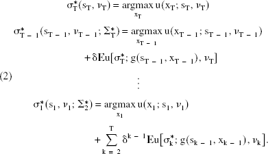
\begin{matrix} σ_{T}^{*} (s_{T}, ν_{T}) = \underset{x_{T}}{a r g m a x} u (x_{T}; s_{T}, ν_{T}) \\ σ_{T - 1}^{*} (s_{T - 1}, ν_{T - 1}; \sum_{T}^{*}) = \underset{x_{T - 1}}{a r g m a x} u (x_{T - 1}; s_{T - 1}, ν_{T - 1}) \\ + δ E u [σ_{T}^{*}; g (s_{T - 1}, x_{T - 1}), ν_{T}] \\ ⋮ \\ \begin{array}{l} \begin{array}{l} \begin{array}{l} σ_{T}^{*} (s_{1}, ν_{1}; \sum_{2}^{*}) = \underset{x_{1}}{a r g m a x} u (x_{1}; s_{1}, ν_{1}) \end{array} \end{array} \end{array} \\ \begin{array}{l} + \sum_{k = 2}^{T} δ^{k - 1} E u [σ_{k}^{*}; g (s_{k - 1}, x_{k - 1}) ν_{k}] . \end{array} \end{matrix}

(2)

In particular, because the utility is concave in x. and the linear combination of concave functions are also concave, backward induction leads to one unique optimal level of x. for each period, beginning with the terminal period. If we take the first-order condition of Equation 1 with respect to x_t, ∀t < T, we have the Euler equation:

\begin{matrix} u_{x} (x_{t}^{*}; s_{t}, ν_{t}) + δ E u_{g} [x_{t + 1}^{*}; g (s_{t}, x_{t}^{*}), ν_{t + 1}] \end{matrix} = 0,

where u_x and u_g are the partial derivatives with respect to × and g, respectively.

Because the Euler equation is linear in δ, given that the utility and the distribution of v are known and x! are the unique and observed optimal consumption levels, the discount factor 8 can then be uniquely identified from the data. Next, we apply this identification strategy to show it is possible to recover the discount rates from a finite sample and to explore the implications of these rates for inference and managerial policy decisions.

Illustrative Application

Consumer Usage Data and Carrier Tariff Structure

A major mobile phone service provider in China supplied the data we use to illustrate the sampling properties of our identification strategy. The data cover the period from September 2004 to January 2005. The data provider accounted for more than 70% of the market share of Chinese mobile phone service market during that time. Initially, this firm used only linear pricing schedules (i.e., consumers were billed on a pay-per-minute basis). In November 2004, the firm offered three-part tariff plans to a randomly selected set of consumers. The firm divided these consumers into multiple groups according to their past usage volumes. The firm then offered each group a respective three-part tariff plan. A consumer could choose the three-part tariff plan or remain on the original pay-per-minute plan.

Tariff structure

Table 2 depicts the pricing structure of the most popular three-part tariff plans, covering 90% of the consumer base. Consumers who enroll in one of the listed plans are allowed a fixed number of free calling minutes in a given calendar month by paying the monthly access fee. When a given consumer places or receives a call, the minutes of the phone call are deducted from the allowance and the consumer does not need to pay for that usage. However, when the monthly allowance is exhausted, the consumer is billed the marginal price for each minute of usage beyond the allowance. There is no “rollover” for these plans (i.e., unused allowance minutes cannot be carried over to next month). At the beginning of next month, the consumer's allowance of free minutes is replenished after paying the new month's access fee. The consumers have different linear rates before the switch. The mean linear rate is .27 with a standard deviation of .09.

Table 2

Three-Part Tariff Plans

Access Fee (CNY)	Allowance (Minutes)	Marginal Price (CNY)	Number of Enrollees	Percentage	Average Linear Rate Before Switch (SD)
98	450	.40	284	50.35	.28 (.10)
128	600	.40	111	19.68	.27 (.09)
168	800	.40	83	14.72	.27 (.07)
218	1100	.36	50	5.92	.25 (.07)
288	1500	.36	21	2.86	.24 (.07)
388	2500	.30	15	2.31	.28 (.04)

Usage data

For the first four months (from September 2004 to December 2004), we observe each consumer's aggregate monthly minute usage and expenditures. However, in the last month (January 2005), we observe call-level consumer records, including the starting time, duration, and expense of each telephone call. The data also include some demographic information, including the age, gender, and zip code of each consumer. Table 3 summarizes the consumers’ average usage levels (normalized by their allowance level) and demographic information. The average usage under both the linear and three-part tariff plans are close.

Table 3

Summary Statistics

	M	SD	Min	Max
Monthly usage under linear plan/allowance level	.92	.46	.02	2.22
Monthly usage under three-part tariff/allowance level	.96	.35	.01	1.63
Female	.16	—	0	1
Rural residency	.41	—	0	1
Age (years)	36.18	7.45	19	58
New customer (enrolled less than 12 months)	.16	.36	0	1

Overage and underage

Underage occurs when consumers do not use all the allowance at the end of a month. In this case, consumers are overpaying in the sense that they have been charged for minutes they do not use. In comparison, overage occurs when usage exceeds the allowance. In this case, consumers again overpay inasmuch as a plan with more allowance minutes normally has a lower average price per allowance minute (Iyengar, Ansari, and Gupta 2007). As a result, consumers who strategically manage the minutes should evidence less underage or overage.

In Figure 1, we plot the histogram of the ratios of minutes used to minutes allowed for the last month of data. The average ratio is close to 1 (.96) under the three-part tariff, suggesting that consumers on average tend to avoid overage or underage. Yet this average behavior belies a large standard deviation (.35). Thus, we next consider whether and how users manage their minutes over the month to comport with the allowance; to the extent this behavior changes as the allowance becomes more salient, evidence is afforded for the strategic use of minutes.

Figure 1

Histogram Of Total Usage Versus Allowance

Strategic minute usage within a month

We consider some model-free evidence that consumers are strategic in their usage of allowance minutes. This evidence is predicated on the notion that minute consumption changes as the distance between minutes used and the allowance becomes small; in particular, consumers begin to conserve minutes as the number of free minutes dwindles and the overage potential increases.

Dividing the last month of the data into five six-day periods, t = 1,…, 5, we compute the ratio of cumulative minutes used to the allowance for each consumer at the end of each six-day period.⁵ Figure 2 portrays a scatter plot of this ratio and its lag value for each period t = 2,…, 5. The line in this figure depicts a nonparametric function relating the ratio and its lag, and the gray band indicates the 95% confidence interval for this function.⁶ A key insight from this figure is that this function is concave when the cumulative usage is within the quota (the ratio in period t − 1 is less than 1). In contrast, when usage exceeds the quota (the ratio in period t − 1 is greater than 1), the line is almost linear. The concavity of the line before exceeding the quota suggests that people decelerate usage as they approach the quota; that is, they begin to ration their minutes to avoid overage. Moreover, those who are far from the quota appear to accelerate usage to avoid underage. In comparison, consumers who have already exceeded the quota do not decelerate (or accelerate) their usage. Instead, they follow some relatively stable usage rates, as might be expected if they no longer faced an intertemporal trade-off in usage. Misra and Nair (2011) and Chung, Steenburgh, and Sudhir (2011) use similar methods to investigate the effect of quota on a salesperson's allocation of efforts across time. They find analogous patterns of dynamic effort allocation in sales force due to quotas.

To test the model's sensitivity to the definition of the six-day period, we also consider the specifications of ten-, five-, and three-day periods. The implied weekly discount factors and price coefficients are statistically equivalent across these different specifications.

We consider both spline and local regression methods, and the results are similar. Figure 2 presents the results from spline method.

Figure 2

The Effect Of Allowance On Minute Usage Over Time

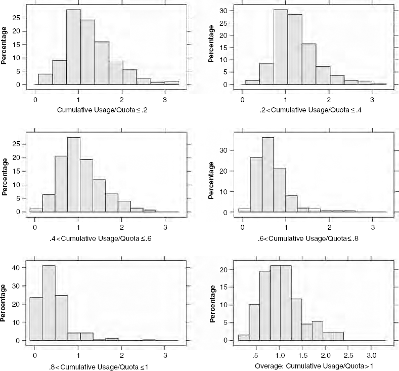
To further elaborate on these insights arising from Figure 2, we consider how usage acceleration (deceleration) changes as people approach their allowance/quota. This acceleration can be summarized by the statistic (Usage during period t)/(Usage during period t − 1). This ratio is analogous to the slope of the line in Figure 2. When the ratio is 1, consumers are neither decelerating nor accelerating use. When the ratio is greater than 1, usage is accelerating, and when it is less than 1, usage is decelerating. We compute this ratio for each person in each period and then, in Figure 3, present a histogram of this minute acceleration measure across users and periods conditioned on users’ distance to the quota. For example, the upper leftmost histogram shows the distribution of usage acceleration observations conditioned on consumer usage at time t − 1 being less than 20% of their allowance. Figure 3 indicates that consumers’ usage decelerates as they approach their allowance. Furthermore, when the consumer reaches an overage situation (in which there is no longer an intertemporal trade-off in usage), the slopes average approximately 1, indicating a stable usage rate. These observations are consistent with Figure 2. Overall, we conclude that there is some model-free evidence of strategic behavior on the part of consumers.

Figure 3

Usage Change Over Time

Model

Utility under the Linear Pricing Plan

In this section, we first specify the consumer utility for consumption under a linear pricing plan and derive the optimal level of consumption. We then extend the analysis to the case of the three-part tariff plan. Similar to Lambrecht, Seim, and Skiera (2007), we begin by assuming that consumer i derives utility from phone usage and the consumption of a composite outside product (numeraire). To be specific,

\begin{matrix} u_{it} (x_{it}, z_{it}) \end{matrix} = (\frac{d_{it}}{b} x_{it} - \frac{1}{2 b} x_{it}^{2}) + z_{it},

(3)

\begin{matrix} subject to z_{it} = y_{i} - p_{i 0} x_{it}, \\ d_{it}, b > 0 \end{matrix}

(4)

where t = 1, 2,…, T are the periods within a month;⁷ x_it is the minutes of phone usage during period t; p_i0 is the linear price rate of consumer i before switching to the three-part tariff; z_it is the consumption of the numeraire;⁸ y_i is the income; d_it/b is the linear component of minute usage utility; and (−1/2b) is its quadratic effect.

We use t to index periods within a month and T to index months.

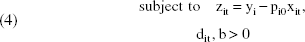
The budget constraint in Equation 4 normalizes the price of the outside good to one, effectively turning it into the numeraire. The purpose of this normalization is twofold. First, it normalizes the marginal utility of income (or numeraire) to one. Because we do not observe consumer churning or variation in plan choices due to income effect in the data, the identification of the marginal utility of income is infeasible. Such a normalization treatment for the purpose of identification is similar to Narayanan, Chintagunta, and Miravete (2007) and Ascarza, Lambrecht, and Vilcassim (2012). Second, it transforms the consumption of minutes into a dollar metric in comparison to the numeraire, making its interpretation more meaningful.

Consumer i chooses the optimal levels of phone usage x_it and numeraire consumption z_it so as to maximize his or her total utility subject to the budget constraint. Substituting the budget constraint Equation 4 into Equation 3, we can rewrite the utility function as follows:

u_{it} [x_{it}, z (x_{it})] = \frac{d_{it} x_{it}}{b} - \frac{x_{it}^{2}}{2 b} + y_{i} - p_{i 0} x_{it} .

(5)

Solving the maximization problem of Equation 5 yields the optimal consumption

\begin{matrix} x_{it}^{*} = {\begin{array}{l} 0, & if d_{it} - {bp}_{i 0} < 0 \\ d_{it} - {bp}_{i0}, & if d_{it} - {bp}_{i 0} \geq 0. \end{array} \end{matrix}

(6)

The foregoing equation clarifies the interpretation of (1) b as the price sensitivity and (2) d_it as the baseline consumption level under the linear pricing plan as it represents a fixed shift in the demand curve as well as the minute consumption level when p_i0 = 0 (Lambrecht, Seim, and Skiera 2007). Following Narayanan, Chintagunta, and Miravete (2007) and Lambrecht, Seim, and Skiera (2007), we further allow baseline consumption, d_it, to be affected by consumer characteristics, D_i, and a random shock v_it:

\begin{matrix} d_{it} = \exp (D_{i}^{'} α) + ν_{it}, \end{matrix}

(7)

where α is a vector of parameters and v_it ∼ N(0, ζ²) is exogenously i.i.d. across consumers and periods.⁹ Sources of the shock may include technical problems with the consumer's phone set or coverage that limit the phone usage; unexpected events that require extra communications with others; and so on. Although the random shocks are unknown to the researchers, the consumer observes the shocks at the beginning of each period, before deciding his or her usage levels accordingly. Given that all consumers in the data set are experienced users, we assume that the distribution of the shocks is known to the consumer.¹⁰ Summing optimal period consumptions within the same month T yields the optimal total minutes consumed within a month as

q_{iτ} = \sum_{t = 1}^{T} x_{it}^{*} .

The exponential function ensures that, on average, d_it > 0. A related concern with the use of a normal distribution assumption for the random shocks is that the baseline demand, d_it, may become negative. One approach is to consider a truncated normal distribution. However, this is computationally costly. Thus, we instead assume that the magnitude of v_it (standard deviation) is small compared with exp(D'_i α), so a normal distribution is a good approximation of a truncated normal distribution. This assumption is consistent with the estimation results.

Although this assumption is not material for the static model because the error is revealed before the usage decision, the assumption becomes important under the context of the three-part tariff when future shocks become relevant to current period consumptions.

Utility under the three-part tariff plan

The three-part tariff plan can be described as the triple {F, A, p}, where F is the fixed access fee, A is the allowance amount, and p is the marginal price after the consumer exhausts the allowance. With regard to period utility and budget constraint, at period t during a given month, consumer i has a utility level

\begin{array}{l} u_{i t} [x_{i t}, z (x_{i t}); s_{i t}, ν_{i t}] = \frac{d_{i t} x_{i t}}{b} - \frac{x_{i t}^{2}}{2 b} + z_{i t} (x_{i t}), \\ s u b j e c t t o z_{i t} (x_{i t}) = y_{i} - C (x_{i t}) \end{array}

\begin{array}{l} C (x_{i t}) = {\begin{array}{l} ({\sum^{​}}_{t - 1}^{k = 1} x_{i k} + x_{i t} - A) p I_{{\sum^{​}}_{t - 1}^{k = 1} x_{i k} + x_{i t} > A}, \\ i f {\sum^{​}}_{t - 1}^{k = 1} x_{i k} < A \\ p x_{i t} i f {\sum^{​}}_{t - 1}^{k = 1} x_{i k} \geq A \end{array} \\ d_{i t} = \exp (D_{i}^{'} α) + ν_{i t}, \end{array}

(8)

where s_it is a vector containing state variables at period t that include (1) cumulative usage up to period t − 1, Σ^t-1_k=1 x_ik and (2) period t (or the distance to the terminal period). Among these state variables, the cumulative usage is endogenous and the period t is exogenous. I_{Σt-1k=1 xjk + xjt > A} is an indicator, which takes the value of 1 if Σ^t-1_k=1 x_ik + x_it > A and 0 if otherwise. Note that the fixed access fee F does not enter the period budget constraint because it is essentially a sunk cost. It does not affect the optimal decision at period t as long as the choice is not a corner solution. Substituting the budget constraint to Equation 8, we can rewrite the period utility as follows:

u_{it} [x_{it}, y_{i} - C (x_{it}); s_{it}, ν_{it}] = (\frac{d_{it} x_{it}}{b} - \frac{x_{it}^{2}}{2 b}) + y_{i} - C (x_{it}) .

(9)

Similar to the period utility under the linear pricing plan, we assume that d_it is affected by the random shock v_it and v_it ∼ N(0, ζ²), where v_it is observed by consumer i at the beginning of period t, before making the decision of minute consumption.

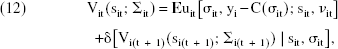
With regard to total discounted utility, because a consumer's current minute consumption may affect his or her future marginal price, the consumer aims to maximize the total discounted utility by optimizing consumption over time. In particular, we can write the total discounted utility at period t ≤ T − 1 as follows:

U_{it} (u_{it}, u_{i (t + 1)}, \dots, u_{iT}) \equiv E (u_{it} + \sum_{k = 1}^{T - t} δ^{k} u_{i (t + k)}),

where δ ∈ [0, 1], representing the discount factor.¹¹

We also estimate a model with an additional hyperbolic discount factor. We do not find strong support for the existence of hyperbolic discounting in our context. Such a result is consistent with Chevalier and Goolsbee (2005) and Dubé, Hitsch, and Jindal (2010). Although time-inconsistent preferences and, thus, hyperbolic discounting exist (Angeletos et al. 2001), they may not be universal in all contexts.

We model the consumer's minute usage decision as the dynamic optimization problem of a Markov decision process (MDP) such that the decision rule of minute usage of period t depends only on the then-current state vector s_it (Rust 1994) and the random shock v_it. To facilitate the exposition, we first define x_it = σ_it ≡ σ_it(s_it, v_it) as the decision rule of consumer i at period t, depending on the state variables s_it and random shock. We also define Σ_it ≡ (σ_it, σ_{i(t + 1}), …, σ_iT) as a decision rule profile for this MDP from period t onward; this profile includes a set of decision rules that dictate current and future consumptions. In addition, we denote V_it(s_it; Σ_it) as the expected continuation utility at period t conditioned on s_it and Σ_it. Because of the finite horizon of this MDP, we can define V_it recursively as follows: The expected utility of the terminal period T for a given s_iT is

V_{iT} (s_{iT}; Σ_{iT}) \equiv E u_{iT} [σ_{iT,} y_{i} - C (σ_{iT}); s_{iT}, ν_{iT}],

(10)

where

C_{(σ_{iT})} = {\begin{array}{l} (\sum_{k = 1}^{T - 1} x_{ik} + σ_{iT} - A) {pI}_{\sum_{k = 1}^{T - 1} x_{ik} + σ_{iT} > A}, \\ if \sum_{k = 1}^{T - 1} x_{ik} < A \\ {pσ}_{iT} if \sum_{k = 1}^{T - 1} x_{ik} \geq A, \end{array}

(11)

where the expectation is taken over the random shock v_iT. Then, we can recursively write the continuation utility function V_it at period t < T as follows:

\begin{matrix} V_{it} (s_{it}; Σ_{it}) =E u_{it} [σ_{it} {,y}_{i} - C (σ_{it}); s_{it}, ν_{it}] \\ + δ [V_{i (t + 1)} (s_{i (t + 1)}; Σ_{i (t + 1)}) | s_{it}, σ_{it}], \end{matrix}

(12)

where

C (σ_{it}) = {\begin{array}{l} (\sum_{k = 1}^{t - 1} x_{ik} + σ_{it} - A) {pI}_{\sum_{k = 1}^{t - 1} x_{ik} + σ_{it} > A}, \\ if \sum_{k = 1}^{t - 1} x_{ik} < A \\ {pσ}_{it}, if \sum_{k = 1}^{t - 1} x_{ik} \geq A, \end{array}

(13)

where the expectation is taken over the random shock v_it. Furthermore, given s_it, v_it, and σ_it(s_it, v_it), the state transition π(s_{i(t + 1)} | s_it, σ_it) is deterministic such that Σ^t_{k = 1} x_ik = Σ^t-1_k=1 x_ik + σ_it, and the consumer is one period closer to the terminal period T.

We further recursively define the optimal decision rule profile $\sum_{it}^{*} \equiv (σ_{it}^{*}, σ_{i(t+1)}^{*}, \dots, σ_{iT}^{*})$ , beginning with the terminal period as

\begin{matrix} σ_{iT}^{*} \end{matrix} = \underset{σ_{iT}}{argmax} u_{iT} [σ_{iT}, y_{i} - C (σ_{iT}); s_{iT}, ν_{iT}],

(14)

and we can recursively define the optimal decision rule of period t < T as

\begin{array}{l} σ_{it}^{*} = \underset{σ_{it}}{argmax} u_{it} [σ_{it}, y_{i} - C (σ_{it}); s_{it}, ν_{it}] \\ + δ [V_{i (t + 1)} (s_{i (t + 1)}; \sum_{i (t + 1)}^{*}) | s_{it}, σ_{it}] . \end{array}

(15)

Estimation

Static Decisions

Consumers make static consumption decisions under (1) the linear pricing plans and (2) the terminal period of the three-part tariff plan. We discuss the likelihood function separately for each case.

Minutes usage under the linear pricing plans

For a given month T under the linear pricing plans, we observe consumer i's characteristics D_i. In our specific application, D_i includes (1) age, (2) the consumer's tenure with the firm, (3) gender, and (4) whether the consumer lives in a rural or urban area.

We also observe individual consumer monthly aggregate usage q_iτ = Σ_t x^*_t.¹² As we show in Appendix B, while there is no closed form for the distribution of q_iτ, the distribution can be approximated by a normal distribution. As a result, we can write down the likelihood function of consumer i for the minutes usage under linear pricing plans:

\begin{matrix} L_{i \cdot Linear} = \prod_{τ} \tilde{f} (q_{iτ} | Ω), \end{matrix}

(16)

where

\tilde{f} (\cdot)

is the approximation density function of q_iτ detailed in Appendix B and Ω ≡ {α, b, ζ} (i.e., the utility parameters and the distribution of random shocks).

Note that for the linear pricing plans, we observe q_iτ only and not the individual x^*_it.

Minutes usage in terminal period T under the three-part tariff

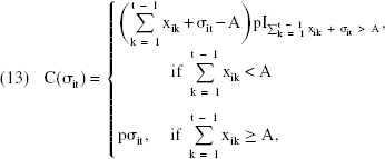
In the terminal period T, the consumption becomes a static decision given that the allowance will be reset the next month. Thus, we can solve the optimal minute consumption strategy σ^*_iT such that

σ_{iT}^{*} = {\begin{array}{l} d_{iT} - bp, & if \sum_{t = 1}^{T - 1} x_{it} + d_{iT} - bp > A \\ d_{iT}, & if \sum_{t = 1}^{T - 1} x_{it} + d_{iT} < A \\ A - \sum_{t = 1}^{T - 1} x_{it}, & if \sum_{t = 1}^{T - 1} x_{it} + d_{iT} - bp \leq A \\ \leq \sum_{t = 1}^{T - 1} x_{it} + d_{iT} . \end{array}

(17)

The first component of Equation 17 accounts for the situation under which the consumer faces a positive marginal price after her cumulative usage exceeds the allowance. The second component represents the situation in which the consumer's cumulative usage is less than the allowance and the marginal price is zero. The third component represents the situation in which the cumulative usage under the optimal σ^*_iT exceeds the allowance at a zero marginal price but falls below the allowance with a positive marginal price. We follow Lambrecht, Seim, and Skiera (2007) and set the optimal usage under such a situation at a mass point σ^*_iT = A − Σ^T-1_t=1 x_it.

According to Equation 17, the density of each observed consumption level x_iT conditioned on σ^{^*}_iT can be written as

\begin{array}{l} f_{T} (x_{iT} | σ_{iT}^{*}, Ω) \\ = {\begin{array}{l} \begin{array}{l} f (x_{iT} = d_{it} - bp) & if \sum_{t = 1}^{T} x_{it} > A \end{array} \\ \begin{array}{l} f (x_{iT} = d_{iT}) & if \sum_{t = 1}^{T} x_{it} < A \end{array} \\ \Pr (\sum_{t = 1}^{T - 1} x_{it} + d_{iT} - bp \leq A \leq \sum_{t = 1}^{T - 1} x_{it} + d_{iT}) \\ if \sum_{t = 1}^{T} x_{it} = A, \end{array} \end{array}

(18)

and the likelihood for consumer i in the terminal period T is

L_{i \cdot Terminal} = f_{T} (x_{iT} | σ_{iT}^{*}, Ω) .

(19)

Dynamic Decisions

Under the three-part tariff, decisions become dynamic for periods t < T. As the result of the dynamic nature of the consumption decision, the discount factor δ enters the data-generating process and thus the estimation. Because there is no closed form solution to the optimal decision rule in the dynamic decision context, a likelihood function based on observed x_it and Σ^*_it becomes infeasible. Instead, we implement a numerical approximation method to establish a simulated likelihood function for estimation. This approximation method contains two steps: (1) using the Gauss-Hermite quadrature method to approximate the value function V_it at a grid of state points and interpolating V_it at the remaining state points using regression and (2) simulating the density for each observed x_it using V_it from the previous step. We elaborate each step next.

Approximating and interpolating V_it(s_it; Σ^*_it)

Using backward recursion and simulation, it is possible to numerically evaluate the value function under the optimal strategy Σ^*_it specified in Equations 15 and 17. Specifically, beginning with the terminal period T:

Pick ns = 250 random draws of state points Σ^T-1_k=1 x_ik to construct a grid (i.e., the cumulative minute usage at the beginning of period T).

For each grid point that we draw, conditioned on Ω, the continuation value function V_iT(s_iT) is approximated as ${\tilde{v}}_{iT} (s_{iT})$ using the Gauss-Hermite quadrature method with nr = 15 nodes (Judd 1998); on each of the nodes, the optimal minute consumption level x^*_iT(s_iT, v_iT) is calculated using Equation 17.

For state points that are not drawn, in line with the value functions obtained on the grid from the previous step, we use a spline interpolation to approximate their values.

Then, for period t < T, we have the following backward recursion steps:

Pick ns = 250 random draws of state points Σ^t-1_k=1 x_ik to construct a grid (i.e., the cumulative minute usage at the beginning of period t).

For each grid point, conditioned on Ω, δ, and the Ṽ_{i(t + 1)}, the continuation value function V_it(s_it) can be approximated as Ṽ_it(s_it) using the Gauss-Hermite quadrature method with nr = 15 nodes; on each of the nodes, we calculate the optimal minute consumption level x_it^*(s_it, v_it) using the following equation:

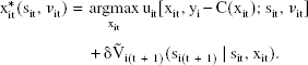
\begin{array}{l} x_{it}^{*} (s_{it}, ν_{it}) & = & \underset{x_{it}}{argmax} u_{it} [x_{it}, y_{i} - C (x_{it}); s_{it}, ν_{it}] \\ + δ {\tilde{V}}_{i (t + 1)} (s_{i (t + 1)} | s_{it}, x_{it}) . \end{array}

For state points that are not drawn, in line with the continuation functions obtained on the grid from the previous step, we use a spline interpolation to approximate their values.

Simulating the density of observed x_it, ${\tilde{f}}_{it}$ (x_it | s_it, Ω, δ)

For each x_it observed in the data and its corresponding state point s_it, we use the following steps to simulate its density:

Draw nr_density = 100 random shocks v_it.

For each random draw of v_it and the observed s_it, calculate the optimal minute consumption by solving the following equation:

\begin{array}{l} x_{it}^{*} (s_{it}, ν_{it}) & = & \underset{x_{it}}{argmax} u_{it} [x_{it}, y_{i} - C (x_{it}); s_{it}, ν_{it}] \\ + δ {\tilde{V}}_{i (t + 1)} (s_{i (t + 1)} | s_{it}, x_{it}) . \end{array}

Using the calculated nr_density = 100 optimal x^*_it (s_it, v_it), simulate ${\tilde{f}}_{it}$ (·), the density of the observed x_it, using the Gaussian kernel density estimator.

With the simulated densities for all observed x_it, we are able to write a likelihood function for consumer i such that

L_{i} = \prod_{t} {\tilde{f}}_{it} (x_{it} | s_{it}, Ω, δ) .

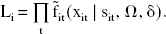
We use maximum likelihood estimation to estimate the parameters. The total likelihood function is

L = \prod_{i} L_{i} \times L_{i \cdot Terminal} \times L_{i \cdot Linear} .

Inference of the Utility Parameters

In this section, we provide an informal discussion of the inference of the utility parameters. Parameters that construct our model can be categorized into two sets. The first set of parameters appear under both the linear pricing plan and the three-part tariff plan, including Ω ≡ {α, b, ζ} (i.e., the utility parameters and the distribution of random shocks). The second set of parameters, δ, only affect the demand under the dynamic setting. In essence, the parameters Ω ≡ {α, b, ζ} are identified from choices under the linear plan and the terminal period of the three-part tariff, where there are no dynamics involved. Conditioned on Ω, we then recover the discount factor δ.

The consumption decisions under the linear plans and the terminal period of the three-part tariff have no dynamics involved. In addition to individual consumption across time, we further observe the following information under the linear plan and the terminal period of the three-part tariff: •

Different linear prices across individual consumers;

•

Depending on whether a consumer has exhausted his or her allowance at the beginning of the terminal period, variation in marginal prices across individuals; and

•

Variation in demographic characteristics across individuals.

The variation in consumption across and within consumers over time, conditioned on the variation in prices and demographics, enables us to identify α and b. Together, α, b prices, and demographics determine the mean levels of consumptions of each consumer over time. The observed deviations from these mean levels across consumers and time identify ζ, the standard deviation of the random shocks v_it.

Monte Carlo Simulation

To evidence the identification approach detailed in the section “Identification of Discount Factors with Static Data” and show that it is possible to recover discount rates from sample data, we employ a Monte Carlo simulation. Using the same consumption model as in our empirical illustration, we simulate three data sets with 50, 75, and 100 customers. To be consistent with the empirical application, in this simulation, each customer makes consumption decisions over five periods. We set the satiation level parameter d = 100, the price sensitivity b = 1, the standard deviation of the random shock ζ = .5, and the discount factor δ = .9. Each data set has both static data and dynamic data.

We report the results in Tables 4, 5, and 6. From the results, we observe the following:

Table 4

Monte Carlo Simulation, N = 50

	One-Step with All Data	Static Data Only	Two-Step	Three-Part Tariff Data Only	Linear Pricing Data and Three-Part Tariff Without Last Period Data	Three-Part Tariff Without Last Period Data
Satiation d = 100	99.58 (.79)	100.55 (.87)	100.55 (.87)	101.10 (1.29)	100.88 (1.03)	150.55 (21.54)
Price b = 1	.94 (.18)	.92 (.20)	.92 (.20)	.90 (.30)	.91 (.28)	2.11 (1.54)
SD of shocks ζ = .5	.51 (.03)	.48 (.03)	.48 (.03)	.55 (.10)	.55 (.08)	1.02 (.50)
Discount factor δ = .9	.88 (.10)	—	.88 (.14)	.89 (.17)	.92 (.15)	.71 (.37)

Notes: Bold values indicate significance at 95% level.

Table 5

Monte Carlo Simulation, N = 75

	One-Step with All Data	Static Data Only	Two-Step	Three-Part Tariff Data Only	Linear Pricing Data and Three-Part Tariff Without Last Period Data	Three-Part Tariff Without Last Period Data (Does Not Converge)
Satiation d = 100	99.89 (0.66)	99.59 (.83)	99.59 (.83)	101.00 (1.08)	100.60 (.99)	—
Price b = 1	.95 (.15)	1.01 (.19)	1.01 (.19)	.93 (.25)	.94 (.22)	—
SD of shocks ζ = .5	.51 (.02)	.51 (.02)	.51 (.02)	.54 (.10)	.53 (.07)	—
Discount factor δ = .9	.91 (.07)	—	.89 (.11)	.92 (.12)	.91 (.11)	—

Notes: Bold values indicate significance at 95% level.

Table 6

Monte Carlo Simulation, N = 100

	One-Step with All Data	Static Data Only	Two-Step	Three-Part Tariff Data Only	Linear Pricing Data and Three-Part Tariff Without Last Period Data	Three-Part Tariff Without Last Period Data
Satiation d = 100	100.15 (.60)	100.41 (.72)	100.41 (.72)	100.95 (.98)	100.59 (.95)	133.11 (25.80)
Price b = 1	.99 (.13)	.99 (.15)	.99 (.15)	.95 (.21)	.97 (.20)	2.01 (1.21)
SD of shocks ζ = .5	.49 (.02)	.49 (.02)	.49 (.02)	.52 (.09)	.52 (.05)	.70 (.55)
Discount factor δ = .9	.89 (.06)	—	.89 (.08)	.91 (.10)	.91 (.08)	.88 (.50)

Notes: Bold values indicate significance at 95% level.

•

Estimating utility with static and dynamic data (Column 1): Using the complete data, estimates of the discount factor and the preference coefficients are statistically indistinguishable from their true values, well within the 95% confidence interval of the true values.

•

Estimating preference parameters using only static data (Column 2): Using only the terminal period of three-part tariff and the linear pricing data, we assess whether preferences can be identified without dynamic usage data. The results indicate that the preference estimates are statistically indistinguishable from their true values, suggesting that the static data are sufficient to infer utility.

•

Estimating the preference parameters and discount factors using a two-step approach (Column 3): In this analysis, we illustrate the identification strategy using a two-step approach. Specifically, we estimate the preference parameters using linear pricing data and the last period of the three-part tariff (as in the preceding step). Conditioned on the preference estimates, in the second step, we then estimate the discount factor using the three-part tariff data, excluding the last period. The preference parameters and discount factor in this two-step approach are statistically equivalent to those estimated jointly in one single step (Column 1). However, the one-step approach is more efficient than two-step approach (Column 3).

•

Estimating the preference parameters and discount rates using only a portion of the static data: Building on the insights we obtained from the previous two steps, this analysis further clarifies the role of static data in identification. Specifically, we estimate the model by pooling static data and dynamic data together. However, for the static data, we either use (1) the linear pricing data or (2) the last period of the three-part tariff data (rather than using both). The results appear in Columns 4 and 5. We find that the preference and discount factor in both cases are statistically equivalent to those estimated with all static data. This finding suggests that the discount factor can be recovered when there are at least some static data to augment the dynamic data. With more data, the estimate of the discount factor becomes more efficient (Columns 4 and 5 vs. Columns 1 and 2).

•

In cases in which the preference and discount factor parameter are identified, more observations under both static and dynamic settings lead to more efficient estimates (Columns 1–5). Moreover, pooling static and dynamic data yields more precise estimates for utility (Column 1 vs. Column 3).

•

The model cannot recover the discount factor when no static data are available (Column 6). –

One of the simulations does not converge (sample size = 75; see Table 5).

–

When the model converges, the price coefficient and discount factor are insignificant, and the satiation level and random shock have greater sampling variance relative to the identified models.

–

In contrast to the case in which the discount factor is identified, more data cannot improve the efficiency of estimates.

•

To assess potential parameter biases when the discount factor is misspecified to be .995, we reestimate our model using this rate on the simulated data for N = 100. The satiation level d and random shock standard deviation ζ are still statistically indistinguishable from the true value $(\hat{d} = 99.33, SE(\hat{d})= . 33; \hat{ζ} = .47, SE(\hat{ζ})= . 02)$ . However, the price parameter b is underestimated ( $\hat{b} = .53$ , SE = .18). The intuition behind the bias is as follows: The higher discount factor implies that consumers excessively substitute future consumption for current within-allowance consumption. Given that future over-allowance consumption is costly, the model compensates by lowering price sensitivity to generate the same level of overall utility for the future consumption occasion. Consequently, the smaller price coefficients imply that the overage charge has less impact on future utility; as a result, there is no need for the consumer to make the trade-off between consumptions across time.

In conclusion, the simulations exemplify the validity of the proposed identification strategy and the potential for misspecification of the discount rate to induce parameter bias.

Results

In this section, we detail the results of our model estimation in the field context described in the “Illustrative Application” section. Whereas the foregoing simulation strategy illustrates the validity of our identification strategy and its ability to uncover the discount factor, the field application is useful in showing that (1) we can estimate discount factors in an actual field setting and (2) the estimated rate is different than commonly assumed in our context. Moreover, as we discuss in the “Managerial Implications” section, this difference can have a material consequence for the inference of the utility parameters, and these biases in utility estimates affect implied policy decisions of firms.

Our sample includes the 284 consumers (50% of the observations) who select the three-part tariff plan with a monthly access fee of 98 RMB (approximately $14), an allowance of 450 minutes, and a marginal price of .4 RMB (see Table 2). We first report the results of our base model and then explore how these estimates are affected by the availability of static data.¹³ As robustness checks, we conclude this section by considering (1) alternative specifications to our continuous specification of heterogeneity, (2) an alternative model of pricing dynamics wherein consumers account for minute usage when billed rather than when used, and (3) potential selection bias.

A separate analysis using 83 consumers (access fee = 168 RMB, allowance of 800 minutes) suggests that our key results are not an artifact of the sample selected.

Parameter Estimates

Table 7 reports the parameter estimates. Considering the utility estimates first, our price estimates imply that a user would cut monthly consumption by approximately 11 minutes for each unit price increase. We also find that rural consumers value the minute consumption marginally higher than urban residents, probably due to their relatively limited access to alternative communication methods such as landlines and the Internet. We also find that female consumers have a higher baseline consumption rate than male consumers.

Table 7

Estimates Of Model Parameters

	Estimate (SE)
Satiation
Constant	4.85 (.13)
Price (cent)	2.15 (.02)
New customer	−.03 (.02)
Age	.04 (.04)
Age²	−.01 (.04)
Rural residency	.03 (.01)
Female	.06 (.02)
SD of shocks	7.46 (2.05)
Weekly discount factor	.90 (.05)

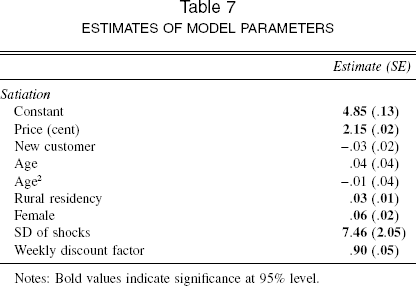
Notes: Bold values indicate significance at 95% level.

Turning to the estimate for discount factor, the estimated weekly discount factor is .9 with a 95% confidence interval of (.78, .97).¹⁴ The corresponding weekly interest rate is 1.11 with a 95% confidence interval of (1.03, 1.28). This discount factor is statistically lower than those typically assumed in structural modeling studies (M = .983; see Table 1). Placing this result in perspective, our estimates indicate that a consumer values an immediate one-minute phone call at the beginning of the month the same as a future call of one minute and 34 seconds at the end of the month. In contrast, a weekly discount factor of .995 implies that a consumer values a one-minute phone call at the beginning of the month to be equal to a one-minute and one additional second at the end of the month (under the assumption of a constant pricing rate). The implication in our model is that consumers would be hesitant to make the latter trade but willing to make the former.¹⁵

We reparameterize the discount factors as δ = exp(π)/[1 + exp(π)] during estimation.

This estimate corresponds to a high annual interest rate of 22,640%. Consumers evidence high levels of impatience in some settings. Warner and Pleeter (2001) find that annual discount factors vary between 0 and .58 (annual interest rate > [1 × 10¹⁴]%) in a field study by observing how agents trade off current and future payoffs. In experimental settings, researchers also find that discount factors may approach zero (e.g., Kirby and Marakovic 1995; Madden et al. 1997; Petry and Casarella 1999). For a more detailed discussion, see Frederick, Loewenstein, and O'Donoghue (2002).

The Effect of Static Data on Inference

As in the case of the simulation, we consider how static data affect inference in our sample of field data (see Table 8). Overall, the findings are consistent with those in our Monte Carlo simulation—namely, that it is difficult to infer discount factors without static data and that more information improves the efficiency of our estimates.

Table 8

Robustness Check: Identification

	Static Data Only	Two-Step	Three-Part Tariff Data Only	Linear Pricing Data and Three-Part Tariff Without Last Period Data	Three-Part Tariff Without Last Period Data	Three-Part Tariff Data Only with Ten-Day Period Definition	All Data with Ten-Day Period Definition
Constant	4.92 (.19)	4.92 (.19)	5.15 (.52)	5.07 (.45)	3.99 (1.26)	9.12 (1.26)	7.89 (.81)
Price (cent)	2.21 (.05)	2.21 (.05)	2.03 (.14)	2.13 (.09)	1.50 (1.00)	1.73 (1.41)	2.09 (.10)
New consumer	−.05 (.03)	−.05 (.03)	−.01 (.11)	−.02 (.10)	.10 (.10)	−.02 (.08)	−.04 (.07)
Age	.02 (.05)	.02 (.05)	.06 (.24)	.05 (.23)	.11 (.30)	.02 (.14)	.01 (.10)
Age²	−.004 (.06)	−.004 (.06)	−.09 (.26)	−.05 (.21)	−.01 (.29)	−.05 (.15)	−.05 (.16)
Rural residency	.04 (.01)	.04 (.01)	.03 (.04)	.01 (.02)	−.03 (.08)	.04 (.07)	.05 (.03)
Female	.04 (.02)	.04 (.02)	.091 (.046)	.11 (.05)	.21 (.39)	.33 (.08)	.10 (.09)
SD of shocks	7.75 (2.28)	7.75 (2.28)	7.50 (3.81)	7.59 (2.91)	9.91 (3.60)	9.58 (4.32)	9.99 (3.90)
Weekly discount factor	—	.89 (.09)	.92 (.13)	.92 (.11)	.95 (.52)	.85 (.55).

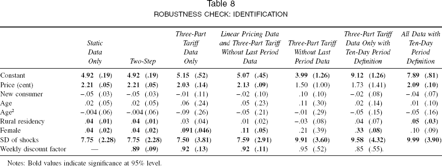
Notes: Bold values indicate significance at 95% level.

In particular, we note that the model cannot recover the discount factor when no static data are available (Table 8, Column 5). Reflective of identification issues, when estimating the model on three-part tariff data without the last period or linear data, the estimation algorithm takes a much longer time to converge even though fewer data are used in estimation (approximately 2.5 times less than the pooling case). More important, the discount factor estimate has a much larger variance (Column 5 in Table 8). The discount factor takes the median of .95 and a standard error of .52. We implement two likelihood ratio tests for H₀: δ = 0 and H₀: δ = 1. In both tests, we cannot reject the null hypotheses; that is, we cannot determine the discount factor without the static data.

Robustness Checks

In this section, we consider several robustness checks to assess how inference regarding the discount rate in our sample might be affected by the interval used for aggregating the data, our assumptions about heterogeneity, and the timing of the payment. We then discuss selection effects.

Data aggregation

We consider the potential effect of temporal aggregation of data on our model estimates. This robustness check demonstrates the effect of data aggregation on the identification of discount rates and preferences (ten-day, five-day, and three-day). The five-day and three-day results are similar to the results reported here; therefore, we focus on the ten-day results. As indicated in Columns 6 and 7 of Table 8, we cannot recover preferences and discount rates using the ten-day intervals unless we use both the static and dynamic data. These results suggest that (1) by reducing the number of observations and the concavity evidenced in Figure 2 (from which we infer intertemporal trade-offs in demand), data aggregation leads to a decrease in the efficiency of the parameter estimates and (2) this problem can be addressed to some degree by using the static data.

Heterogeneity

As another robustness check, we explore the effect of our parametric assumption regarding consumer utility on the inferred discount factor. To do this, we estimate the model consumer by consumer (by combining static and dynamic data), thereby allowing all users to have different preferences and discount factors. We find the median discount factor across consumers to be .87 (SD = .26), similar to the level estimated under the homogenous model.¹⁶ We also consider a latent class mixture model. This analysis yielded two segments. The first, comprising 85% of the consumers, evidenced a discount rate of .89 (SE = .04), while the smaller segment rate was estimated to be .92 (SE = .05). Overall, it appears that our discount factor estimates are robust to our specification of heterogeneity.

Recognizing the potential for small sample problems arising from maximum likelihood estimation in our panel (we have limited observations per customer for inference), we use simulated data to explore this potential. Specifically, we generate data using the parameters estimated from our homogeneous model. In one case, we generate 1000 static observations per consumer. In another case, we use 3 static observations (as observed in the data) to supplement the dynamic data. We then proceed to estimate our model consumer by consumer for both simulated data sets. The estimates from the larger sample are statistically equivalent to those in the current study (price Mdn = 2.17, SD = .10; discount Mdn = .91, SD = .11). We further find a small degree of small sample bias for the three-observation case. The price coefficients are slightly overestimated (Mdn = 2.99, SD = .79) and the discount factors are slightly underestimated (Mdn = .84, SD = .28); but they are both still statistically equivalent to those in the current study (2.15 and .90). The simulation suggests that the small bias is not sufficient to change our conclusion that the static data enable identification of discount rates. This is consistent with our Monte Carlo simulation results.

Payment timing

Note that Equations 5 and 9 presume that consumers account for minutes at the time they are transacted rather than when they are billed. To explore this assumption, we consider some model-free tests. Specifically, when the “mental accounting” of the expense is concurrent with the billing date and the pricing plan is linear, the usage decision becomes dynamic in the early periods of the month. This is because the consumption x_it in period t will affect the total payment in period T, but not the period in which the usage occurs. This implies a downward trend in optimal consumption within the month because future payments are discounted more steeply in earlier periods. If the payment only materializes in period T, the utilities in periods t and T become

\begin{matrix} u_{it} = \frac{d_{it} x_{it}}{b} - \frac{x_{it}^{2}}{2 b} + y_{i} \\ u_{iT} = \frac{d_{iT} x_{iT}}{b} - \frac{x_{iT}^{2}}{2 b} + y_{i} - p_{i 0} \sum_{k = 1}^{T} x_{ik} . \end{matrix}

The optimization problem of period t is

x_{it}^{*} = \underset{x_{it}}{argmax} u_{it} + δ^{T - t} E_{d} u_{iT} .

Taking first-order condition to solve $X_{it}^{*}$ , we can show that

x_{it}^{*} = d_{it} - {bδ}^{T - t} p_{i0} .

This implies that, on average, the minute usage should drop over time if the payment only materialized in the utility function of period T. This observation suggests some model-free tests of whether consumers budget for minutes at the point of consumption or at the payment: •

Model-free evidence 1: Although our data for the first few months do not include call-by-call observations under the linear pricing plan, sales agents contacted consumers in month 3 to offer the three-part tariff option. The timing of the call for each consumer was random, and the consumers had no foresight of the call. Importantly for our immediate concern, data were collected regarding the total minute consumption under the linear plan before the offer. These data enable us to calculate average weekly minute consumption across consumers up to the week of the switch. If the consumers account for payments at the terminal period T, usage rates over time should decrease on average. Figure 4 is a box plot that depicts the averages of weekly usages of consumers who switched during the same week. It indicates no downward trend in consumption. This pattern is inconsistent with a mental accounting of expense at the time of billing.

Figure 4

Average Usage Over Weeks

•

Model-free evidence 2: In the bottom right-hand panel of Figure 3, when consumers exceed the quota, the three-part tariff becomes a linear plan. If there is a downward trend in consumption, we should likewise see the histogram skewed toward 0, reflective of usage deceleration. However, according to Figure 3, the consumption rate is centered on 1, which is also inconsistent with the mental accounting of expense at the time of billing.

•

Model comparison: In addition to these model-free tests, we further consider a third test based on the three-part tariff data. We estimate a dynamic model similar to the base model but with the payment only entering in period T. The results indicate that the price sensitivity is not significant and the discount factor, though similar to our estimate in the current study, has a large standard error. Model fit deteriorates as measured by Bayesian information criterion (BIC) (9470.12 vs. 9511.30) and mean absolute percentage error (MAPE) (.14 vs. .23).

Accordingly, the data seem to be more consistent with the “mental accounting” of payment at time of consumption than with payment at time of billing.

Selection

Our data include only consumers who switch price schedules. Although the static and dynamic data are sufficient to identify the preference and discounting, as shown in the Monte Carlo simulation, to the extent a consumer's adoption decision could be endogenous, the estimates in this field application may not be generalized to the overall population due to potential selection bias. To explore the potential selection effects, we estimate the model separately for consumers who chose two different three-part tariff plans (450 minutes plan vs. 800 minutes plan). Table 9 presents the results.

Table 9

Robustness Check: Selection

	Plan 800 Minutes	Plan 450 Minutes (Estimates in the Current Study)
Constant	5.05 (.33)	4.85 (.13)
Price (cent)	2.91 (.04)	2.15 (.02)
New customer	−.10 (.05)	−.03 (.02)
Age	.05 (.11)	.04 (.04)
Age²	−.02 (.05)	−.01 (.04)
Rural residency	.10 (.03)	.03 (.01)
Female	.19 (.07)	.06 (.02)
SD of shocks	8.85 (2.01)	7.46 (2.05)
Weekly discount factor	.88 (.06)	.90 (.05)

Notes: Bold values indicate significance at 95% level.

Of note, the discount factors for consumers selecting each plan are statistically similar (.90 vs. .88). In contrast, the preference estimates are different. In particular, those who chose the 450-minute plan have a lower baseline consumption (a smaller constant estimate) and lower price sensitivity. This is intuitive because (1) consumers with lower baseline consumption needs are more likely to enroll in a lower allowance plan and (2) consumers with lower price sensitivity are more likely to enroll in a lower allowance plan because they care less about overage charges.

This robustness check merely shows that the estimates are conditional on a set of consumers that self-select into a pricing scheme that induces a forward-looking incentive (as in Goettler and Clay 2011). However, one key implication of this exercise is that the findings are consistent with the conjecture that selection plays a greater role in consumption utility than discounting.

Managerial Implications

The dynamics of consumer behavior may have substantial impact on firm strategic decisions and revenues. In this section, we build on the broad literature pertaining to plan choice over months for telephony or Internet services (e.g., Grubb and Osborne 2012; Iyengar, Ansari, and Gupta 2007; Lambrecht and Skiera 2006; Lambrecht, Seim, and Skiera 2007; Narayanan, Chintagunta, and Miravete 2007) to explore (1) the implications of within-month pricing policy on carrier revenue and (2) how discount rates affect these policies.

Usage Prediction and Intertemporal Substitution Pattern

Biased price effects

To assess the potential bias in model estimates arising from specifying the commonly employed discount factor of .995 rather than using the estimated discount factor, we reestimate the model by fixing the discount factor to .995. While there is little impact on most estimates, we find the price coefficients to be underestimated (have smaller absolute magnitudes) by 16%. The price coefficient becomes 1.81 (vs. 2.15 in Table 7), with a standard error of .03. This underestimation of price effects is consistent with the findings of the Monte Carlo simulation we performed.

Biased forecasts

To ascertain how well the model fits the data and resulting intertemporal substitution pattern, we calculate the in-sample MAPE, BIC, and mean percentage error (MPE) across time under both the estimated discount rate and the assumed weekly discount factor of .995. The MAPE measures a model's overall accuracy of fitting the data, while the MPE indicates bias in model predictions. Tables 10 and 11 depict the results.

According to Table 10, the fit under the .995 discount factor is universally worse than the fit under the estimated coefficients across time as measured by both MAPE and BIC. To develop a better sense of why the higher discount factor performs more poorly, we next turn to the MPE. Based on Table 11, there is no obvious forecasting bias from using the higher discount rate when summing across all periods, and yet aggregating across time obscures the patterns in intertemporal substitution. When setting the discount factor at .995, the demand in the first four periods is underestimated, and the demand in the terminal period is overestimated. This bias occurs because consumers are more impatient than what δ = .995 implies. As a result, in the early periods, when the allowance has not been exhausted, impatient consumers consume more than predicted under the .995 discount factor. Furthermore, consumers are more price sensitive than the .995 discount factor case implies (recall that the price coefficient is underestimated under the .995 discount factor). As a result, consumers in overage (roughly coincident with the last period) evidence lower consumption than predicted under the .995 discount factor.

Table 10

Mape Comparison

	MAPE
Estimated Discount Factors (BIC: 9470.12)
First four periods	.14
Final period	.16
Monthly aggregate	.14
Discount Factor Set to .995 (BIC: 9499.95)
First four periods	.17
Final period	.21
Monthly aggregate	.18

Notes: Likelihood ratio test χ² = 37.42, H₀: δ = .995 is rejected.

Table 11

Mpe Comparison

	MPE
Estimated Discount Factors
First four periods	.02
Final period	→ 0
Monthly aggregate	.02
Discount Factor Set to .995
First four periods	−.09
Final period	.02
Monthly aggregate	−.03

Although the difference between the estimated discount factor (M = .90, with a 95% confidence interval of (.78, .97)) and .995 seems negligible, the effect on the forecast results are highly significant. This is because the joint distributions of all of the coefficients differ considerably under the two scenarios. The inflated discount factor .995 also causes biased estimates of preference, especially downward-biased price sensitivity (2.15 vs. 1.81).

Elasticities

To ascertain how consumers’ minutes usage varies under alternative allowance and the marginal price levels, we compute their monthly minutes demand changes for both the estimated discount factor and .995. Table 12 presents the results. The elasticities in Table 12 suggest that the .995 discount factor leads to an underestimation of the effect of allowances and price on usage (i.e., users are not as price sensitive as it implies when the discount factor is set to .995). If consumers were to actually have a discount factor of .995, they would be more forward looking than they are under the actual discount rates we estimate. As a result, the more forward-looking consumers implied by .995 should conserve minutes so as not to pay overage in later periods. Because they do not actually conserve minutes, the model with a .995 discount factor needs to rationalize the observed overage. It does so by estimating a relatively lower sensitivity to price and allowance; a lower price and allowance sensitivity means that consumers do not mind paying overage as much and have lower elasticities.

Table 12

Demand Elasticities

	Demand Elasticity with Regard to Price Overall	Demand Elasticity with Regard to Price After Overage
Estimated discount factors	−.07 (−.09, −.05)	−.19 (−.21,−.16)
Discount factor set to .995	−.06 (−.07, −.04)	−.13 (−.14,−.11)

	Demand Elasticity with Regard to Allowance
Estimated discount factors	24 (.21, .26)
Discount factor set to .995	.18 (.15, .19)

Notes: 95% confidence intervals are in parentheses. Bold values indicate that the biases are significant (p > .05).

Alternative Pricing Schedule

According to our communication with the data provider, its process of picking the three-part tariffs in this field study is ad hoc: There was no price optimization consideration. As a result, the focal three-part tariff is not likely to be optimal for the firm in terms of maximizing its revenue. To access the potential for revenue improvement, we create a grid of alternative allowance and price levels. For each combination of allowance and price, we calculate the percentage of revenue change at the end of the month.¹⁷ Table 13 reports the results.¹⁸

Table 13

Revenue Percentage Change Under Alternative Pricing Schedules (δ = −.90)

Allowance (Minutes)	Marginal Price
Allowance (Minutes)	.34	.36	.38	.40	.42	.44	.46
300	−.11	−.06	−.05	−.03	−.09	−.15	−.08
325	.05	.19	.27	.20	.07	−.01	−.05
350	.05	.23	.30	.36	.29	.25	.18
375	.89	.93	.98	.72	.69	.55	.40
400	.92	1.11	.97	.96	.83	.77	.61
425	.82	.95	.94	.80	.73	.68	.51
450	.01	.27	.22	0	.16	.11	.07
475	−.18	.12	−.15	−.22	−.30	−.33	−.51
500	−.21	−.14	−.23	−.25	−.33	−.48	−.61

Notes: The best alternative is in boldface.

Note that we do not model plan choice because there are no plan choice data available. To ensure that the presented price/allowance changes do not lead to consumers leaving the company or opting for a different plan, we calculate consumer welfare for each point on the grid as measured by consumers’ total discounted utility. We then compare it with the welfare level under the original plan. None of the welfare changes is significantly different from zero; thus, we do not believe that the recommended policies will result in substantial plan switching even though these changes benefit the firm. Furthermore, the company had a significant market share, and there was no cell phone number portability in China until October 2010 (ChinaTechNews.com 2010). Consequently, we conclude that (1) the new price structures in Table 12 are unlikely to have caused large consumer churning and plan switching and (2) the effect of competitive response is likely to be modest.

To account for sampling error when computing the revenue changes, we sample 100 sets of values from the estimates distribution. We then calculate the revenues using these sampled estimates. The table presents the median values.

Table 13 includes the current plan (allowance = 450 minutes, price = RMB.40). Surrounding the current plan, each column from left to right represents a 2-cent change in the marginal price for minutes in overage and each row from top to bottom stands for a 25-minute change in the allowance. A lower allowance enhances the possibility of overage; and a moderately decreased price tends to increase the consumption level under the overage situation. The optimal combination of allowance and marginal price is 400 minutes and .36 RMB. The revenue of the firm would increase by 1.11% under this alternative pricing schedule. To the extent that similar exercises can be implemented across all groups of consumers, the revenue increase would be considerable.

As shown previously, under the discount factor of .995, the model may lead to biased estimates of coefficients and elasticities. To determine whether such biases may lead to inaccurate policy recommendations, we recreate the same grid but calculate the revenue changes using the estimates under the .995 discount factor. As Table 14 indicates, with the .995 discount factor, the model generates notably different pricing plan recommendations. Because the assumed discount factor is much higher, to enhance consumers’ likelihood of overage, the allowance levels would be much lower. As a result, under the .995 discount factor, the optimal allowance level becomes 325 instead of 400. Moreover, because the price sensitivities are underestimated, the optimal price would be higher. This effect leads to the optimal price changes from .36 to .38. In short, the firm sets its allowance too low and its marginal price somewhat high, thereby overcharging its consumers when using the standard practice of setting discount rates.

Table 14

Revenue Percentage Change Under Alternative Pricing Schedules (δ = .995)

Allowance (Minutes)	Marginal Price
Allowance (Minutes)	.34	.36	.38	.40	.42	.44	.46
300	.59	.79	.92	.72	.61	.55	.39
325	.65	.80	.96	.88	.77	.73	.64
350	.48	.57	.71	.94	.83	.80	.75
375	.43	.47	.54	.68	.58	.44	.39
400	.11	.23	.33	.49	.44	.40	.36
425	.08	.14	.19	.21	.21	.18	.17
450	−.11	−.07	−.02	0	−.01	−.05	−.08
475	−.22	−.21	−.17	−.23	−.31	−.34	−.38
500	−.39	−.36	−.33	−.41	−.46	−.51	−.57

Notes: The best alternative is in boldface.

The predicted revenue gains also significantly differ between the two scenarios, δ = .90 vs. δ = .995. For each grid point, we calculate the predicted revenue difference between the two scenarios. As in Figure 5 shows, the percentage differences can be substantial. By implementing the pricing plans as suggested by the model with δ = .995, the firm would forgo revenue gains. For example, with an allowance of 400 and a price of .36 (where δ = .90), the firm's revenue improvement would be 1.11% (95% confidence interval (.80%, 1.43%)). However, if the firm used δ = .995, it would predict that the revenue could only improve by .23% (95% confidence interval (−.05%, .67%)). In comparison, with δ = .995, the firm would adopt the “optimal” plan with an allowance of 325 and a price of .38 and expect a revenue improvement of .96% (95% confidence interval (.66%, 1.23%)). However, the actual revenue improvement would only be .27% (95% confidence interval (−.01%, .53%)). Such a suboptimal pricing level would reduce the potential gains by 76% relative to the optimal pricing level.

Figure 5

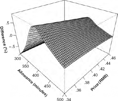
Revenue Prediction Differences: δ =.90 Versus δ = .995

Conclusion

Due to the ability to capture the trade-off between long-term and short-term goals, the application of dynamic structural models to consumer and firm decision making has become increasingly widespread. However, dynamic structural models face a fundamental identification problem— namely, that the preference, the state transition, and the discount factor are confounded and become difficult to identify simultaneously. If the rate is misspecified, inferences about agent behavior might be misleading, and the implied policies for improving agent welfare might be suboptimal.

We advance the literature on identifying discount factors by using field data to measure them. Specifically, we estimate a dynamic structural model using consumers’ cell phone usage data. The data contain observations of consumers’ cell phone consumptions under both static and dynamic settings. Using the static data, we first identify consumers’ utilities and the distribution of random consumption shocks. Conditioned on the identified utilities and random shocks, we then recover the discount factor using the dynamic data. The identification strategy proposed may have more general applications in contexts beyond the cell phone pricing strategy we consider herein. The identification of discount factors is possible if researchers observe consumers making continuous decisions under both static and dynamic settings. Such contexts may include loyalty programs, markdown pricing during clearance and seasonal sales, some finite duration auctions, and perishable goods such as ticket sales.

Findings suggest that the discount factor in our specific context (.90) is significantly below those commonly assumed in the literature (.995). As a consequence, price effects are underestimated in our application. Moreover, the higher rate leads to a mistaken presumption that more minutes would be saved for later use, leading to a 29% increase in the MAPE in model fit. The attendant consequences for pricing policy are notable, leading to pricing recommendations that are generally too high and would lower potential revenue gains by 76%.

The inherent complexity of dynamic structural models often requires simplifications that correspondingly represent future research opportunities. Our model is no exception. First, our study focuses on a specific consumption context with a small focal group of consumers over a specific duration. Therefore, the results may not generalize to other contexts involving different consumers, decisions, or decision durations. Thus, more research is necessary to generalize the degree to which discount rates are an inherent trait or the degree to which they are context dependent. For example, it would be fruitful to consider how discount rates might vary in practice when considering different contexts of intertemporal consumption; do consumers invoke the same level of patience when making choices over years as they do when making decisions over days?

Second, two potential sources of selection bias exist in our field study. The first arises from the firm's choices of consumers to participate in the plans. Per our discussion with the firm's managers, consumer selection was randomized, so this form of selection bias is not germane. The second selection bias arises from the consumer's decision of whether to adopt the three-part tariff plan that was offered. The decision to adopt the plan can be correlated with both preferences and discounting behavior. As such, our estimates should be interpreted conditional on plan selection (as in Goettler and Clay 2011), limiting the generalizability of estimated rates to the overall consumer population of the company. As a result, another area of interest is to extend our research into the domain of plan choice to broaden insights regarding the distribution of discount rates across the population. Third, our identification strategy is based on a dynamic model with continuous controls. We discuss the set identification conjecture for discrete decisions in Appendix A. A more formal investigation on the identification on discrete decision dynamic models would be a challenging but significant extension.

In summary, the current study is the first (to our knowledge) to provide field study–based evidence regarding the nature of discount rates that obviate the need for structural assumptions or exclusion restrictions to identify discount rates. Consistent with Dubé, Hitsch, and Jindal (2010) and Ishihara (2010), we find evidence that discount rates are substantially lower than those used in practice and that this difference is material from a policy perspective. Given the widespread use of dynamic models in marketing and economics, we hope our analysis will spark future work to pin down how such intertemporal trade-offs are made in practice.

Footnotes

The Identification of the Discount Factor

Appendix A details the identification of the discount factor when the utility and random shock distribution are known. We extend the discussion of finite horizon case in the “Identification of Discount Factors with Static Data” section to a more general infinite horizon case. We show that, conditioned on the utility and random shock distribution being identified by the static data, the discount factor is identified. We also provide a conjecture about the identification of discrete choice dynamic decision process with finite horizon.

The Distribution of Monthly Minutes usage q iτ Under Linear Pricing Plan

Because we only observe the monthly minute consumption q_iτ = Σ_tx_it^* but not each respective x_it^*, we need to find the likelihood of q_iτ. As discussed in Equation 6, the optimal minutes usage at period t, x_it^*, may take two values, 0 (if d_it-bp_i0 ≤ 0) and d_it − bp_i0 (if d_it − bp_i0 > 0). Because d_it = exp(D'_i α) + v_it and v_it ∼ N(0, ζ²), x_it^* follows a normal distribution N[exp(D'_i α) − bp_i0,ζ²] that is truncated at zero. Thus, the density of x_it^* is (B1)

\begin{matrix} f (x_{it}^{*}) = \frac{1}{ζ} ϕ (\frac{x_{it}^{*} - μ_{i}}{ζ}) / [1 - Φ (- \frac{μ_{i}}{ζ})], \\ where μ_{i} = \exp (D_{t}^{'} α) - {bp}_{i 0} . \end{matrix}

The monthly minute consumption q_iτ = Σ_tx_it^* can then be written as the summation of a series truncated normal random variables with the same truncation at zero. Although there is no closed form for the distribution of q_iτ, if the occurrence of zero minute consumption for any period is nearly zero $[Pr (x_{it}^{*} > 0) \to 1, \forall_{t}]$ , q_iτ can be approximated well by a normal density function whose mean is T × μ_i and the variance as $T \times ζ_{g}^{2}$ .¹⁹ Intuitively, although $x_{it}^{*}$ is a truncated normal random variable, if ${Pr(x}_{it}^{*} > 0)$ is nearly one, the truncation becomes moot and the distribution of $x_{it}^{*}$ can be approximated well by a normal distribution. The summation of a series of i.i.d. normal random variables is also normally distributed. We implement a Monte Carlo simulation using this approximation. The parameters are recovered with reasonable accuracy. As a robustness check to this approximation, we also use a Kernel estimator to compute the density in the Monte Carlo simulation (Härdle and Linton 1994). The results are similar to the ones using the approximation, but the Kernel estimation is much more computationally demanding.

The analytical proof of the validity of this approximation and Monte Carlo simulation results are available on request.

References

Ackerberg

Daniel A.

(2003), “Advertising, Learning, and Consumer Choice in Experience Good Markets: An Empirical Examination,” International Economic Review, 44 (3), 1007–1040.

Allcott

Hunt

, and Wozny

Nathan

(2011), “Gasoline Prices, Fuel Economy, and the Energy Paradox,” working paper, MIT Center for Energy and Environmental Research Policy.

Angeletos

George-Marios

, Laibson

David

, Repetto

Andrea

, Tobacman

Jeremy

, and Weinberg

Stephen

(2001), “The Hyperbolic Consumption Model: Calibration, Simulation, and Empirical Evaluation,” Journal of Economic Perspectives, 15 (3), 47–68.

Ascarza

Eva

, Lambrecht

Anja

, and Vilcassim

Naufel

(2012), “When Talk Is ‘Free’: An Analysis of Subscriber Behavior Under Two- and Three-Part Tariffs,” working paper, Columbia Business School.

Busse

Meghan R.

, Christopher

R. Knittel

, and Zettelmeyer

Florian

(2012), “Are Consumers Myopic? Evidence from New and Used Car Purchases,” The American Economic Review, forthcoming.

Chevalier

Judith

, and Goolsbee

Austan

(2005), “Are Durable Goods Consumers Forward-Looking? Evidence from College Textbooks,” NBER Working Paper No. 11421.

ChinaTechNews.com (2010), “China to Start Trial of Mobile Phone Number Portability in October 2010,” (August 17), (accessed August 3, 2012), [available at http://www.chinatechnews.com/2010/08/17/12425-china-to-start-trial-of-mobile-phone-number-portability-in-october-2010].

Chung

Doug

, Steenburgh

Thomas

, and Sudhir

(2011), “Do Bonuses Enhance Sales Productivity? A Dynamic Structural Analysis of Bonus-Based Compensation Plans,” Working Paper No. 11-041, Harvard Business School.

Dubé

Jean-Pierre

, Günter

J. Hitsch

, and Chintagunta

Pradeep

(2010), “Tipping and Concentration in Markets with Indirect Network Effects,” Marketing Science, 29 (2), 216–49.

10.

Dubé

Jean-Pierre

, Günter

J. Hitsch

, and Jindal

Pranav

(2010), “Estimating Durable Goods Adoption Decisions from Stated Preference Data,” working paper, Booth School of Business, University of Chicago.

11.

Dubin

Jeffrey A.

, and Daniel

L. McFadden

(1984), “An Econometric Analysis of Residential Electric Appliance Holdings and Consumption,” Econometrica, 52 (2), 345–62.

12.

Erdem

Tülin

, and Michael

P. Keane

(1996), “Decision-Making Under Uncertainty: Capturing Dynamic Brand Choice Processes in Turbulent Consumer Goods Markets,” Marketing Science, 15 (1), 1–20.

13.

Fang

Hanming

, and Wang

Yang

(2012), “Estimating Dynamic Discrete Choice Models with Hyperbolic Discounting, with an Application to Mammography Decisions,” NBER Working Paper No. 17384.

14.

Frederick

Shane

, Loewenstein

George

, and O'Donoghue

Ted

(2002), “Time Discounting and Time Preference: A Critical Review,” Journal of Economic Literature, 40 (2), 351–401.

15.

Goettler

Ronald L.

, and Clay

Karen

(2011), “Tariff Choice with Consumer Learning and Switching Costs,” Journal of Marketing Research, 48 (August) 633–52.

16.

Gordon

Brett R.

(2009), “A Dynamic Model of Consumer Replacement Cycles in the PC Processor Industry,” Marketing Science, 28 (5), 846–67.

17.

Grubb

Michael D.

, and Osborne

Matthew

(2012), “Cellular Service Demand: Biased Beliefs, Learning, and Bill Shock,” working paper, MIT Sloan School of Management, Massachusetts Institute of Technology.

18.

Härdle

Wolfgang

, and Linton

Oliver

(1994), “Applied Nonparametric Methods, in Handbook of Econometrics, Vol. 4, Engle

Robert

, and McFadden

Daniel

, eds. Amsterdam: Elsevier Science, 2295–2339.

19.

Harrison

Glenn W.

, Morten

I. Lau

, and Melonie

B. Williams

(2002), “Estimating Individual Discount Rates in Denmark: A Field Experiment,” The American Economic Review, 92 (5), 1606–1617.

20.

Hartmann

Wesley R.

(2006), “Intertemporal Effects of Consumption and Their Implications for Demand Elasticity Estimates,” Quantitative Marketing and Economics, 4 (4), 325–49.

21.

Hartmann

Wesley R.

, and Harikesh

S. Nair

(2010), “Retail Competition and the Dynamics of Demand for Tied Goods,” Marketing Science, 29 (2), 366–86.

22.

Hausman

Jerry A.

(1979), “Individual Discount Rates and the Purchase and Utilization of Energy-Using Durables,” The Bell Journal of Economics, 10 (1), 33–54.

23.

Hendel

Igal

, and Nevo

Aviv

(2006), “Measuring the Implications of Sales and Consumer Inventory Behavior,” Econometrica, 74 (6), 1637–73.

24.

Hotz

V. Joseph

, and Robert

A. Miller

(1993), “Conditional Choice Probabilities and the Estimation of Dynamic Models,” The Review of Economic Studies, 60 (3), 497–529.

25.

Ishihara

Masakazu

(2010), “Dynamic Demand for New and Used Durable Goods Without Physical Depreciation: The Case of Japanese Video Games,” working paper, Stern School of Business, New York University.

26.

Iyengar

Raghuram

, Ansari

Asim

, and Gupta

Sunil

(2007), “A Model of Consumer Learning for Service Quality and Usage,” Journal of Marketing Research, 44 (November) 529–44.

27.

Judd

Kenneth L.

(1998), Numerical Methods in Economics. Boston: MIT Press.

28.

Kim

Jun

, Albuquerque

Paulo

, and Bart

J. Bronnenberg

(2010), “Online Demand Under Limited Consumer Search,” Marketing Science, 29 (6), 1001–1023.

29.

Kirby

Kris N.

, and Nino

N. Marakovic

(1995), “Modeling Myopic Decisions: Evidence for Hyperbolic Delay-Discounting Within Subjects and Amounts,” Organizational Behavior and Human Decision Processes, 64 (1), 22–30.

30.

Lambrecht

Anja

, Seim

Katja

, and Skiera

Bernd

(2007), “Does Uncertainty Matter? Consumer Behavior Under Three-Part Tariffs,” Marketing Science, 26 (5), 698–710.

31.

Lambrecht

Anja

, and Skiera

Bernd

(2006), “Paying Too Much and Being Happy About It: Existence, Causes, and Consequences of Tariff-Choice Biases,” Journal of Marketing Research, 43 (May), 212–23.

32.

Lee

Robin S.

(2011), “Dynamic Demand Estimation in Platform and Two-Sided Markets: The Welfare Cost of Software Incompatibility,” working paper, Stern School of Business, New York University.

33.

Madden

Gregory J.

, Nancy

M. Petry

, Gary

J. Badger

, and Warren

K. Bickel

(1997), “Impulsive and Self-Control Choices in Opioid-Dependent Patients and Non-Drug-Using Control Participants: Drug and Monetary Rewards,” Experimental and Clinical Psychopharmacology, 5 (3), 256–62.

34.

Magnac

Thierry

, and Thesmar

David

(2002), “Identifying Dynamic Discrete Decision Processes,” Econometrica, 70 (2), 801–816.

35.

Misra

Sanjog

, and Nair

Harikesh

(2011), “A Structural Model of Sales-Force Compensation Dynamics: Estimation and Field Implementation,” Quantitative Marketing and Economics, 9 (3), 211–25.

36.

Narayanan

Sridhar

, Chintagunta

Pradeep

, and Miravete

Eugenio

(2007), “The Role of Self Selection, Usage Uncertainty and Learning in the Demand for Local Telephone Service,” Quantitative Marketing and Economics, 5 (1), 1–34.

37.

Petry

Nancy M.

, and Casarella

Thomas

(1999), “Excessive Discounting of Delayed Rewards in Substance Abusers with Gambling Problems,” Drug and Alcohol Dependence, 56 (1), 25–32.

38.

Rust

John

(1987), “Optimal Replacement of GMC Bus Engines: An Empirical Model of Harold Zurcher,” Econometrica: Journal of the Econometric Society, 55 (5), 999–1033.

39.

Rust

John

(1994), “Structural Estimation of Markov Decision Processes,” in Handbook of Econometrics, Vol. 4, Robert

F. Engle

, and Daniel

L. McFadden

, eds. Amsterdam: Elsevier Science, 3082–3143.

40.

Stokey

Nancy L.

, and Robert

E. Lucas

(1989), Recursive Methods in Economic Dynamics. Cambridge, MA: Harvard University Press.

41.

Sun

Baohong

(2005), “Promotion Effect on Endogenous Consumption,” Marketing Science, 24 (3), 430–43.

42.

Warner

John T.

, and Pleeter

Saul

(2001), “The Personal Discount Rate: Evidence from Military Downsizing Programs,” The American Economic Review, 91 (1), 33–53.

43.

Zeithammer

Robert

(2006), Forward-Looking Bidding in Online Auctions,” Journal of Marketing Research, 43 (August), 462–76.

Determining Consumers’ Discount Rates with Field Studies

Abstract

Keywords

Relevant Literature

Identification of Discount Factors with Static Data

Illustrative Application

Consumer Usage Data and Carrier Tariff Structure

Tariff structure

Usage data

Overage and underage

Strategic minute usage within a month

Model

Utility under the Linear Pricing Plan

Utility under the three-part tariff plan

Estimation

Static Decisions

Minutes usage under the linear pricing plans

Minutes usage in terminal period T under the three-part tariff

Dynamic Decisions

Approximating and interpolating Vit(sit; Σ*it)

Simulating the density of observed xit, f ˜ it (xit | sit, Ω, δ)

Inference of the Utility Parameters

Monte Carlo Simulation

Results

Parameter Estimates

The Effect of Static Data on Inference

Robustness Checks

Data aggregation

Heterogeneity

Payment timing

Selection

Managerial Implications

Usage Prediction and Intertemporal Substitution Pattern

Biased price effects

Biased forecasts

Elasticities

Alternative Pricing Schedule

Conclusion

Footnotes

The Identification of the Discount Factor

The Distribution of Monthly Minutes usage q iτ Under Linear Pricing Plan

References

Approximating and interpolating V_it(s_it; Σ^*_it)

Simulating the density of observed x_it, ${\tilde{f}}_{it}$ (x_it | s_it, Ω, δ)