The Impact of Category Prices on Store Price Image Formation: An Empirical Analysis

Abstract

The authors empirically explore how consumers update beliefs about a store's overall expensiveness. They estimate a learning model of store price image (SPI) formation with the impact of actual prices linked to category characteristics on a unique data set combining consumers’ store visit and purchase information with their price perceptions. The results identify characteristics that drive categories’ store price signaling power for different store formats. “Big ticket” categories with a narrow price range strongly shape consumers’ store price beliefs, whereas (volatile) prices of frequently or deeply promoted categories are less influential. At traditional supermarkets, consumers anchor and elaborate on prices of storable categories bought in large quantities and for which quality differentiation is high. For hard discounters, however, SPI is mostly shaped by frequently bought categories with narrow assortments. Notably, categories’ SPI signaling power is not proportional to their share of wallet at either type of chain. Managers can use these results to identify “Lighthouse” categories that signal low prices, yet make up a small portion of store spending, and in which price cuts do not overly hurt revenue.

Keywords

store price image price perceptions product category characteristics Bayesian learning

Consumers use store price images (SPIs)—holistic constructs that summarize how cheap or expensive stores are— to guide their store choice and purchasing decisions (Arnold, Oum, and Tigert 1983; Hamilton and Chernev 2013; Mazumdar, Raj, and Sinha 2005). A recent Nielsen report indicates that “Good Value for Money is now the most important determinant of grocery store choice” and that “of those consumers who rated ‘good value for money’ as very or quite important when deciding where to do their grocery shopping, 70% said it was important the store had a reputation for being cheaper than competitors—even if, in reality, this was not the case” (Nielsen 2008, p. 4). Given this “power of perception,” managing SPI has become a major concern in retail pricing practice (Hamilton and Chernev 2013). For example, France-based Carrefour, the largest hypermarket chain in the world, has invested more than half a billion dollars in its price image in 2009 alone (Lagorce 2009). As another example, in April 2010, retail giant Wal-Mart cut the prices of 10,000 items in the U.S. market, with the goal of “polishing its discount image” (Bustillo and Martin 2010). In addition, between 2003 and 2005, the leading Dutch supermarket chain Albert Heijn slashed prices in a wide range of categories to restore a more favorable price perception (Van Heerde, Gijsbrechts, and Pauwels 2008).

With retail margins becoming increasingly tight, a critical question for retailers is which product categories are more salient in the consumer SPI formation process and why (Desai and Talukdar 2003; Grewal and Levy 2007). Such knowledge is crucial for the development of category-level pricing policies that create a favorable price perception while maximally preserving store revenue or margins. Previous studies have already considered the effect of (specific) category characteristics on store price beliefs but have done so either conceptually (Hamilton and Chernev 2013) or in an experimental setting (e.g., Alba et al. 1994; Büyükkurt 1986; Desai and Talukdar 2003), which makes it difficult to uncover the dynamics in the SPI formation process. Evidence on how category prices dynamically influence perceived store expensiveness in a real-life setting remains scant.

In this article, we empirically document which product categories are more influential in shaping SPIs over time in a natural setting and explore how previously proposed category characteristics drive these differences. We estimate a dynamic model of SPI formation including category prices on the basis of a unique data set that combines weekly store visits and purchases from a representative panel of households, with semiannual store price perceptions of these same households.¹ The data cover all major Dutch retail chains and contain their weekly prices for nearly 50 product categories over a period of four years. Our focus on category prices is justified by the wide array of categories in a typical grocery store—the prices of which are not likely to be processed by consumers in the same way—and by previous findings that category factors are powerful drivers of price responses and perceptions (Bell, Chiang, and Padmanabhan 1999; Desai and Talukdar 2003). Our focus also fits into a category management perspective and generates guidelines that retailers can put into action. Industry reports have indicated that 84% of retailers cite the opportunity to increase profitability as their motivation for using category management (e.g., Nielsen 2004; Progressive Grocer 2007).

We use the terms “consumer(s)” and “household(s)” interchangeably throughout the article, assuming that the survey respondent is the household member responsible for the household's purchases (i.e., the consumer).

We contribute to the literature in several ways. First, we present a dynamic model of how changes in category prices alter consumers’ SPI and estimate this model on real-life data. Second, we consider a fairly broad set of category drivers and study their effects for two store formats: traditional supermarkets (TSs) and hard discounters (HDs). Third, we explore household differences in category-based SPI learning and show that categories that constitute a large chunk of the household's spending do not necessarily have the highest signaling power. To academics, we offer evidence on how consumers update their store price beliefs from different category prices in different store formats, thereby answering Hamilton and Chernev's (2013) recent call for this type of research. For managers, our results help identify “Lighthouse” categories—that is, categories that create a favorable SPI while constituting only a small portion of the consumers’ sales share at the store (and, thus, in which the direct revenue losses from a price drop will be lower).

In the next section, we discuss relevant background literature. We then describe our unique data set and our statistical model. Subsequently, we present the estimation results, followed by a discussion on managerial implications. We end with conclusions and future research directions.

Background and Conceptual Framework SPI

Formation as a Learning Process

Extant literature has characterized SPI development as a dynamic process. Consumers’ initial perceptions about a store's overall expensiveness are often based on nonprice cues that are readily accessible and expected to correlate with store prices (Alba et al. 1994; Hamilton and Chernev 2013). Examples of these cues are the store's ambiance, its service level, the promotions it advertises, and the assortment it carries (Baker et al. 2002; Büyükkurt 1986; Hamilton and Chernev 2013).

Consumers gradually update their store price beliefs as they visit the store and are exposed to the actual prices charged by that store (Büyükkurt 1986; Feichtinger, Luhmer, and Sorger 1988; Mägi and Julander 2005; Nyström 1970). Such learning may be intentional (i.e., consumers actively look for price cues to update their store price knowledge; e.g., Gauri, Sudhir, and Talukdar 2008; Urbany, Dickson, and Kalapurakal 1996) or incidental (i.e., consumers integrate price signals automatically as they happen to be exposed to them; Desai and Talukdar 2003; Hoch and Deighton 1989; Mazumdar and Monroe 1990). Moreover, although actual prices tend to be most informative for consumers whose SPI is still uncertain (Hamilton and Chernev 2013), even consumers who are knowledgeable about the store's expensiveness are likely to process new incoming price information to keep price beliefs up to date (Desai and Talukdar 2003; Jensen and Grunert 2014; Urbany, Dickson, and Kalapurakal 1996; Vanhuele and Drèze 2002;). Our model builds on these insights.

Impact of Category Prices on SPI updating

Grocery stores carry thousands of items in a multitude of product categories. Accurately assessing the price level of a store is therefore a “daunting task” (Mägi and Julander 2005, p. 320), and because of its sheer complexity, consumers tend to adopt simplifying heuristics (Alba et al. 1994; Mägi and Julander 2005). For example, consumers may be affected by prices of categories they are exposed to but do not actually buy from (Hamilton and Chernev 2013). Moreover, the extent to which category prices are encoded and integrated into overall beliefs is subject to perceptual biases and information processing costs (Hoch and Deighton 1989): consumers’ SPI may be more strongly influenced by category prices that are (1) salient or perceived as important, (2) easy to compare, and/or (3) easy to recall (Desai and Talukdar 2003; Urbany, Dickson, and Kalapurakal 1996).²

“Salience/perceived importance” refers to the likelihood that consumers will be exposed to or pay attention to prices and encode them on the spot. “Ease of comparison” reflects how easy consumers find it to evaluate category prices—that is, to meaningfully compare them with some (internal or external) reference standard at the time of exposure. “Ease of recall” indicates the ease with which consumers can retrieve encoded category prices at a later time.

Figure 1 lists a set of category drivers of SPI signaling value proposed in the literature (e.g., Alba et al. 1994, 1999; Desai and Talukdar 2003; Hamilton and Chernev 2013). We focus on category drivers that are managerially useful (i.e., easy for retailers to identify and incorporate in their pricing strategy) and that are testable in our study. In the following subsections, we briefly discuss these drivers and their potential role in shaping SPIs.

Figure 1

Conceptual Framework: Impact Of Category Prices On Spi

Purchase frequency and quantity

Existing studies have suggested that frequently purchased categories matter more in price image formation (Hamilton and Chernev 2013). Not only are consumers more often exposed to prices in regularly purchased categories, which makes them more salient (Desai and Talukdar 2003) and easier to recall in later price judgments (Alba et al. 1994; Briesch et al. 1997; Pauwels, Srinivasan, and Franses 2007), but they also have more to gain from low prices in those categories (Wakefield and Inman 1993; Urbany, Dickson, and Kalapurakal 1996). Similarly, consumers would attach greater importance to prices in categories that involve higher discretionary spending (i.e., larger volumes per purchase) and make up a greater portion of their shopping basket (Desai and Talukdar 2003; Feichtinger, Luhmer, and Sorger 1988).

Expensiveness and price range

Not surprisingly, several studies have suggested that expensive categories play a larger role in the formation of store price beliefs (Desai and Talukdar 2003; Hamilton and Chernev 2013). “Big ticket” items may attract more attention (Zeithaml 1988), and their prices may be deemed more important, which increases price encoding, elaboration (Desai and Talukdar 2003; Miyazaki, Sprott, and Manning 2000), and ease of recall (Kardes 1994). Prior research has also shown that, in addition to the overall price level, consumers may be sensitive to the range of prices (i.e., the difference between the lowest and highest regular price across the category's stockkeeping units [SKUs]; Alba et al. 1994). In categories with high price dispersion, the stakes appear higher (Briesch et al. 1997; Pauwels, Srinivasan, and Franses 2007; Urbany, Dickson, and Kalapurakal 1996), and the mere presence of a low price may be a cue that prices are low in general (Hamilton and Chernev 2013).

Promotion frequency and depth

Some categories are more often promoted than others, and experimental studies have suggested that this affects the category's importance for SPI formation beyond its regular price (Alba et al. 1994, 1999; Lalwani and Monroe 2005)³: frequent price cuts generate more attention from consumers and trigger more elaborate processing and rehearsal (Desai and Talukdar 2003; Kardes 1994). Researchers have also proposed the magnitude of a category's promotional discounts (i.e., the typical depth of temporal price cuts for a given SKU) as a driver (Alba et al. 1994, 1999; Hamilton and Chernev 2013), with different possible effects. Although deep price cuts (that exceed a threshold) may make category prices more salient (Büyükkurt 1986; Pauwels, Srinivasan, and Franses 2007) and more important for consumers to monitor (Kopalle, Mela, and Marsh 1999; Mela, Gupta, and Lehmann 1997; Mela, Jedidi, and Bowman 1998), they may also introduce uncertainty into consumers’ reference price or “comparison standard” for the category (Gupta and Cooper 1992; Pauwels, Srinivasan, and Franses 2007), thus reducing its signaling role for SPI formation (Büyükkurt 1986; Feichtinger, Luhmer, and Sorger 1988).

Like Nijs et al. (2001), Raju (1992), Bolton (1989), Bell, Chiang, and Padmanabhan (1999), and others, we consider average deal depth and frequency as exogenous, market-level category characteristics. These category factors then moderate the impact of specific marketing actions (including temporary price cuts and feature support by specific retailers at specific times). See our operationalizations in Table 4.

Assortment size and quality differentiation

Scholars have also conjectured that characteristics of the category assortment influence how category prices are integrated into overall store price beliefs (Hamilton and Chernev 2013). Whereas categories with many brands or SKUs tend to be more salient to consumers (Briesch et al. 1997; Desmet and Renaudin 1998)—and, thus, more prominent in SPI formation— the presence of multiple, differently priced brands and packages hampers the establishment of a clear reference price for the category (Hoch and Deighton 1989) (making category prices less powerful signals of the store's overall expensive-ness). Similarly, large perceived quality differences may lower consumers’ focus on price (Steenkamp, Van Heerde, and Geyskens 2010) and impede meaningful category-price comparisons among stores with different assortments (Lynch and Ariely 2000).

Storability

Finally, research has found storability to moderate consumers’ reaction to price cuts in a category (Narasimhan, Neslin, and Sen 1996) as well as their leeway to defer a category purchase (Gijsbrechts, Campo, and Nisol 2008; Krider and Weinberg 2000). As such, it may also affect the role of category prices in building store price beliefs, either positively (consumers may be inclined to monitor prices due to potential savings from stockpiling storable products) or negatively (because buying perishable items cannot easily be postponed or shifted to other-store visits, consumers may view them as “locked in” to the store's expensiveness).

Store Format Differences

As indicated by Hamilton and Chernev (2013), the drivers of SPI beliefs may differ between store formats. In addition to TSs, we consider HD stores (such as Germany-based Aldi and Lidl). Not only have these stores reached high shares in Western Europe (e.g., both Lidl and Aldi feature among the top six retail grocery players; Planet Retail 2014) and impressive growth rates in the United States (Steenkamp and Kumar 2009), but SPI formation at these stores may be very different from traditional chains. First, the types of customers that shop at these two formats differ. Hard discounters primarily attract price-sensitive shoppers who tend to have better store price knowledge (Mägi and Julander 2005) and buy larger baskets on average—characteristics that have been suggested to affect SPI formation (Hamilton and Chernev 2013). Second, the TS and HD formats constitute radically different shopping contexts. Hard discounters are “lean,” no-frills stores that carry far fewer SKUs and hardly any national brands per category. Moreover, being private label (PL) dominated, they have not only much lower average prices but also less price dispersion within categories (Lourenço and Gijsbrechts 2013; Steenkamp and Kumar 2009). As a result, all else being equal, identifying and comparing prices is less challenging at HDs than at TSs (Zielke 2010). Third, the price dynamics at these formats are dramatically different. Whereas traditional chains (in our study) typically follow a hi–lo strategy, HD chains adhere to an everyday-low-price business model with low regular prices rather than promotion deals. Our empirical results shed light on how these forces affect the formation of store price beliefs and, in particular, categories’ SPI signaling power at the two store formats.

Methodology

Setting and Data

For our empirical analysis, we have access to a unique combination of data sets. First, we have information on consumers’ store price perceptions, collected semiannually by GfK from its panel members. The data span a period of four years, from 2002 to 2005, and each of the survey waves was conducted during one week. In the course of that week, a random subsample of panelists were asked to judge the overall price level (along with other characteristics) of the stores they visited in that week. Specifically, after returning from a store visit, at the time they would scan their purchases along with their scanner-panel identification, they answered the question “How do you rate the prices of products in this store?” by scanning the appropriate category on an ordinal scale from 1 (“excellent”) to 9 (“very bad”).⁴ Thus, panel members only evaluated stores they actually visited during the survey week, and a household could rate multiple stores patronized in the course of that week. In addition to store price beliefs, the survey collected panel members’ perceptions on other image components of the stores. Surveys were conducted in weeks 16 and 40 of every year, with an extra survey wave in week 5 of 2004.

Not all panel members who received a request to participate in the survey in a specific wave actually responded. Panelists were given the possibility to opt out after scanning their purchases (the typical response rate was 70%).

Second, for the same panel members and in the same time period, we have scanner panel data on spending at visited stores for all 18 major grocery retail chains in the Netherlands. Two of these chains (Aldi and Lidl) belong to the HD format, and the remaining chains are TSs. We only retain households that are in the panel throughout the observation period and that participated in the survey. Table 1 indicates, for each chain format, the number of panelist responses in each survey wave and the number of shopping trips (across all sample panelists) observed since the previous wave. It shows that the survey responses (and store visits) are balanced over time and that each format is well represented in the data. On average, each household engages in 175 shopping trips (in the course of the 194-week period), provides 11.5 SPI responses, and participates in approximately 7 survey waves (6.85). The average number of different stores rated by a household is 3.0. In total, 11.3% of panelists only rated HD stores, 44.3% only TSs, and 44.4% of the sampled households provided price-image data for stores in both format types.

Table 1

Number Of Spi Survey Evaluations And Store Visits By Wave

	HDs		TSs
Survey Wave	Survey Ratings	Trips Since Previous Wave	Survey Ratings	Trips Since Previous Wave
1	77	N.A.	563	N.A.
2	71	750	556	4,521
3	92	849	556	4,579
4	94	961	508	4,392
5	88	925	519	4,220
6	76	824	502	4,187
7	79	772	450	3,854
8	97	855	462	3,647
9	79	837	393	3,334

Notes: N.A. = not applicable.

Data on actual prices and feature promotions are available by chain⁵ on a weekly basis for 49 product categories identified by GfK (which, together, capture more than 85% of sales in each chain). As for the category prices, we use the same construct as Van Heerde, Gijsbrechts, and Pauwels (2008). First, we calculate the price of a category c in a store s and week t (P_c,st) as a weighted average of the unit price (e.g., price per liter, price per ounce) of the brands in that category, store, and week, using the overall market share of the brands in an initialization period as weights.⁶ Next, to make these prices (expressed in different units for different categories) comparable across categories, we rescale them into a category price index (PI_c,st) for that week and store. Specifically, we calculate ${PI}_{c, st} = P_{c, st} / {\bar{P}}_{c}$ , where ${\bar{P}}_{c}$ is category c's average actual price across all stores during an initialization period (which, in some sense, can be thought of as a “reference price” for the category). Note that because ${\bar{P}}_{c}$ does not vary across periods or stores, it only rescales the absolute prices into common units across categories (see also Van Heerde, Gijsbrechts, and Pauwels 2008) that are easy to interpret: values below (above) 1 indicate that the category has become cheaper (more expensive) in that store and week relative to its average market level in the initial period.

Exceptions are Aldi and Lidl, for which GfK did not provide feature data. Because feature support for grocery items is relatively limited at these stores, we do not expect this limitation to be a problem for our remaining model estimates.

We use an initialization period, rather than the brand sales share in the period itself, to avoid endogeneity in the price constructs: if we used brand shares in the same period as weights, these shares could be higher in weeks with lower brand prices, placing overly high weight on those low prices. Following Van Heerde, Gijsbrechts, and Pauwels (2008), given the volatility of SKU shares within a brand, we first calculate brand prices as unweighted averages of SKU unit prices within the brand and then weigh these brand prices to obtain category-level price measures.

Model of SPI Formation

Basic updating process

Building on previous literature, we model SPI formation as a process of adaptive learning over time (see Alba et al. 1994; Büyükkurt 1986; Feichtinger, Luhmer, and Sorger 1988; Nyström 1970). We use the following notation: i = 1, …, N consumers, s = 1, …, S stores, and c = 1, …, C product categories; T_i > 0 is the number of store visits for consumer i. Because the acquisition of exhaustive price information is prohibitive, consumers will be uncertain in their evaluation of stores’ overall price levels (Desai and Talukdar 2003). Let $S \bar{P} I_{ist-1}$ be consumer i's mean belief about the overall expensiveness of store s at time t - 1, and let σ_{SPIist - 1}² be the uncertainty (variance) of his store price belief. The SPI beliefs (mean and uncertainty) not only are household and store specific but also can change over time. During a store visit in t, the consumer has access to the prices actually charged by the store in different categories (PI_{c, st}, c = 1, …, C). In the spirit of adaptive learning, he would then adjust his mean store price perceptions using some weighted average of his previous store price beliefs and this new price information (Feichtinger, Luhmer, and Sorger 1988; Nyström 1970):

S \bar{P} I_{ist} = w_{0, ist} S \bar{P} I_{ist - 1} + \sum_{c = 1}^{C} w_{c, ist} {PI}_{c,st,}

(1)

where w_0,ist and w_c,ist are consumer i's weights attached to his previous price image about store s and to observed category prices, respectively. Although category prices themselves are not ambiguous, the large amount of price information to be processed creates uncertainty surrounding the price signals (Mägi and Julander 2005). This “imprecision” may result from difficulties in encoding, comparing, or remembering prices for inclusion in SPI, and we further specify its link with household, category, and store characteristics subsequently.

Equation 1 is very general, in the sense that it allows the weights to be consumer, store, period, and (for the price weights) category specific. To make the expression operational, we must impose some structure on the learning process (i.e., on the weights). In line with recent marketing studies (e.g., Erdem, Keane, and Sun 2008; Shin, Misra, and Horsky 2012; see also Erdem and Keane's [1996] seminal paper and Ching, Erdem, and Keane's [2013] up-to-date overview), we adopt a Bayesian framework to capture the updating process.⁷ The Bayesian model offers a simple account of consumer learning that can explain a considerable range of phenomena and has been found to make sensible predictions (Shin, Misra, and Horsky 2012). Moreover, the Bayesian model fits well with the SPI formation process described in the literature (Büyükkurt 1986; Feichtinger, Luhmer, and Sorger 1988; Nyström 1970). Consumers combine their prior SPI beliefs with new price evidence to obtain posterior beliefs (which, in turn, constitute priors for the next update) in such a way that incoming information becomes less important (and SPI beliefs become less uncertain) as they build up experience. This finding is consistent with previous observations that as a store price perception becomes formed, it may be more difficult to change (Desai and Talukdar 2003; Hamilton and Chernev 2013), and that store-profile effects may persist even after exposure to in-store price information (Büyükkurt 1986).

The premise that consumers learn about the overall price level of a store using category prices as (noisy) signals is not at odds with poor recall of product item prices (Dickson and Sawyer 1990). Consumers may hold a distributional belief about prices instead of a point estimate (i.e., learning occurs with uncertainty; see Monroe and Lee 1999). In addition, consumers may encode price stimuli in different ways (Mazumdar and Monroe 1990), as is the case if specific item prices are integrated into SPI for later use without separately encoding each of those prices in absolute terms.

In the Bayesian framework, assuming that consumer i's prior SPI beliefs (in t – 1) and category price signals (in t) are normally distributed (with means $S \bar{P} I_{ist-1}$ and PI_{c, st}, respectively), her posterior belief about the overall expensiveness of store s at time t is normally distributed as well, with mean and variance given by DeGroot (1970):

\begin{array}{l} S \bar{P} I_{ist} = \\ σ_{{SPI}_{ist}}^{2} {\frac{1}{σ_{{SPI}_{ist - 1}}^{2}} S \bar{P} I_{ist - 1} + \sum_{c = 1}^{C} \frac{1}{[1 + (r - 1) F_{c,st}] σ_{η_{c,i}}^{2}} {PI}_{c,st}}, and \end{array}

(2)

σ_{{SPI}_{ist}}^{2} {\frac{1}{σ_{{SPI}_{ist - 1}}^{2}} + \sum_{c = 1}^{C} \frac{1}{[1 + (r - 1) F_{c,st}] σ_{η_{c,i}}^{2}}}^{- 1} .

(3)

In Equation 2, the weights attached to previous and new information are proportional to the “precision” (inverse of the variance) of each piece of information: the precision of the prior belief (i.e., 1/[σSPI_ist–1²]) and, as we explain next, the precision of each category-price signal (i.e., 1/{[1 + (r – 1)F_c,st]σ_ηc,i²}). Accordingly, category prices that have more uncertainty associated with them should be less influential in the integration mechanism (Büyükkurt 1986), which is incorporated in the Bayesian updating process in Equation 2. Moreover, consumers who are more exposed to price information have greater objective and subjective store price knowledge (Magi and Julander 2005); that is, they feel more confident about their judgments. This is captured in Equation 3, which implies that the posterior SPI variance— a combination of the prior belief's variance and the variance of the price signals—decreases over time.⁸

Indeed, drawing on Equation 3, we obtain the posterior precision of the SPI belief as the prior precision plus the sum of the category price-signal precisions, which are both positive numbers.

As Equations 2 and 3 show, the link between SPI and prices is governed by the price-signal precisions, given by 1/{[1 + (r - 1)F_c,st]σ_ηc,i²}. In this expression, σ_ηc,i² is the “intrinsic” category-price signal variance⁹ (which is time and store independent but varies across categories and consumers, as we discuss in the next section), F_c,st is the fraction of products in category c at store s that appear in the store's flyer at time t, and r is a “feature parameter” to be estimated (with 0 < r < 1). The logic behind this expression is as follows. When featured in the store flyer, category prices are more likely to be noted and to contribute to SPI formation. Equations 2 and 3 account for this feature effect by expressing the weight of a category price signal received by consumers at a given store and time as a function of that category's feature intensity at that store and time.¹⁰

The price signal variance σ_ηc,i² is not to be confused with the variance of the actual prices. The latter reflects the variation in the category prices as observed in/used by the store. In contrast, the price signal variance in the Bayesian model (or rather, its inverse) reflects the extent to which price signals are deemed informative of the store's SPI; higher levels of σ_ηc,i² imply that the consumer learns less from prices about the store's expensiveness.

As F_c,st approaches 1 (maximum feature support for category c in store s in t), the category's price weight for the store at that time approaches 1/rσ_{η_c,st}². If F_c,st = 0 (i.e., the category does not appear in the store's flyer), the category's price weight reduces to 1/σ_ηc,i², which is the inverse of its intrinsic signal variance for the household.

Category drivers of SPI learning

As we indicated in the “Background and Conceptual Framework” section, apart from their appearance in the store flyer in a particular period, consumers might not process all category price signals in the same way. To accommodate this possibility, we can “enrich” the traditional Bayesian updating Equations 2 and 3 by specifying the signal precisions as a function of category drivers. In Equations 2 and 3, a higher value of 1/σ_ηc,i² implies that consumer i learns more from the prices of product category c. In line with our conceptualization, we specify the category- and consumer-specific precisions 1/σ_ηc,i² as a function of category characteristics m (some of which are household specific). To accommodate unobserved heterogeneity, we add a random term ξ_c,i, such that

In (\frac{1}{σ_{η_{c,i}}^{2}}) = β_{0} + \sum_{k = 1}^{K} β_{k + 1} {In m}_{k,c,i} + ξ_{c,i,},

(4)

with

ξ_{c, i}, \sim N(0, σ {}_{ξ}^{2})

and k = 1, …, K. The double-log specification guarantees positive signal precisions and makes the coefficients directly interpretable as elasticities. In Equation 4, positive (negative) coefficients correspond to positive (negative) effects on the price-signal precisions, indicating that the corresponding variable enhances (decreases) learning from category prices. Note that for σ_ξ² = 0, r = 1, and

\forall k > 0

: β_k = 0; the proposed model in Equations 2–4 nests a simple specification with category prices as signals and signal precision equal to exp(β₀).

Initialization

Equation 2 is a recursive relation that needs to be initialized. Let $S \bar{P} I_{is0}$ be consumer i's initial mean price belief about store s, with variance σ_{SPI_is0}². As advocated by Hamilton and Chernev (2013) and Buyükkurt (1986), we specify the initial (mean) beliefs about the expensiveness of store s, $S \bar{P} I_{is0}$ , to be a linear function of its perceived non-price cues:

S \bar{P} I_{i s 0} = φ_{0} + \sum_{ℓ = 1}^{L} φ_{ℓ} Z_{ℓ, i s},

(5)

where Z_ℓ, is (ℓ = 1, …, L) are perceived store characteristics other than price that affect the consumer's perception of expensiveness of the store (which we further specify subsequently). Because these nonprice perceptions are household specific, the associated initial price beliefs are as well. We obtain the initial variance for each store as the variance of the initial beliefs across households (for details on the measurement, see Web Appendix A).

Model Estimation

In assessing the parameters of Equations 2–5, we face several challenges. With full information on the consumers’ price image beliefs about the different stores at any point in time (i.e., SPI_ist, the mean and variance of which are given in Equations 2 and 3), we could simply replace $S \bar{P} I_{ist}$ in Equation 2 with this observed value plus a normally distributed error ζ_ist with zero mean (i.e., $S \bar{P} I_{ist} = {SPI}_{ist} + ζ_{ist}$ and, combined with observed store prices and category characteristics, estimate the model parameters. However, such perception data are usually not available. In our setting, we do have access to survey data on scanner panelists’ SPI evaluations at different points in time, but the properties of these data introduce some challenges.

First, the measured price perceptions obtained from the surveys (MSPI_ist) are only ordinal (not interval) scaled. Second, unlike the stores’ category-price information (which is available on a trip-by-trip basis), the SPI data are collected only biannually (i.e., there are typically two survey waves each year), so we do not observe SPI “updates” following each store visit. Third, although the perception data are longitudinal in the sense that survey respondents come from the same panel of households in each survey wave, the perception histories are incomplete: most households provide stated perceptions for only a subset of stores (see the following section for more details). So, even if our data offer a unique opportunity to match households’ scanner panel data (including actual store visits and encountered prices) with store price perception data, they are not without limitations.

To deal with the ordinal scale of the image data, we add an extra layer to the model, which maps the latent, unobserved store price image SPI_ist onto the measured MSPI_ist = j:

α_{j - 1} < {SPI}_{ist} + ε_{ist} \leq α_{j}, j = 1, \dots, J,

(6)

where the α_j are threshold parameters to be estimated and ε_ist is an independent, normally distributed random term, ε_ist ∼ N(0, σ_ε²), which leads to the well-known ordered probit model.

To cope with the missing-data problem, we adopt a Bayesian estimation approach. As indicated by Van Heerde, Mela, and Manchanda (2004), this approach is particularly well suited to deal with incomplete and unevenly spaced data. The model works as follows. For each household–store combination, the household's (unobserved) price belief about the store—and more specifically, its mean and variance—are updated in every period in which the house-hold actually visits the store on the basis of the price signals received in-store at that time. These beliefs are then confronted with the stated store price perceptions only in periods in which a survey measure MSPI_ist is actually available. Thus, the model efficiently uses all available observations: store visits and category price and feature information for all stores and panelists on a weekly basis; price-image survey measures across households, stores, and survey waves; and household-specific and market-level product category characteristics. In summary, the model consists of Equations 2 and 3, the updating equations for the mean and variance of the store price beliefs; Equation 4, which expresses the contribution of the category prices to these beliefs as a function of (household and) category characteristics; Equation 5, which governs the initial values of the store price beliefs; and Equation 6, which maps the ordinal survey measures on to the underlying continuous store price beliefs. To accommodate differences between TS and HD chains, we estimate the model in Equations 2–6 by store format. Web Appendix A provides details on the estimation procedure.

Preliminary Data Analysis and Operationalization of Drivers

Descriptives

Table 2 provides some summary statistics for the SPI data. It displays, for the HDs and the top three TSs, the mean and median rating for each of the nine survey waves and the percentage change in coefficient of variation between subsequent waves. Not only are the differences between stores substantial (with a particularly large gap between TS and HD stores), there are also significant within-store shifts across the survey waves (see also the paired Wilcoxon test results at the bottom of Table 2).

Table 2

Spi Across Waves For The Top Three Tss And Two Hds

	M (Mdn)			Percentage Change in CV from Previous Wave	M (Mdn)		Percentage Change in CV from Previous Wave
Survey Wave	TS1	TS2	TS3	All TS	HD1	HD2	All HDs
1	4.56 (5.0)	4.06 (4.0)	4.34 (4.0)	N.A.	3.17 (3.0)	3.09 (3.0)	N.A.
2	4.63 (5.0)	3.70 (3.0)	4.32 (5.0)	13.1	2.93 (3.0)	3.08 (3.0)	3.6
3	4.66 (5.0)	3.74 (4.0)	4.48 (5.0)	6.9	3.08 (3.0)	3.00 (3.0)	10.8
4	4.86 (5.0)	3.96 (4.0)	4.24 (4.0)	6.5	3.03 (3.0)	3.09 (3.0)	3.2
5	4.52 (5.0)	3.59 (3.0)	4.59 (5.0)	11.7	3.06 (3.0)	3.13 (3.0)	10.0
6	4.36 (4.5)	3.90 (4.0)	4.23 (4.0)	3.2	3.31 (3.0)	2.83 (2.5)	17.6
7	4.41 (5.0)	3.59 (3.0)	4.33 (5.0)	8.0	3.21 (3.0)	3.05 (3.0)	14.2
8	4.27 (4.0)	3.96 (4.0)	4.33 (5.0)	5.7	3.34 (3.0)	3.23 (3.0)	3.6
9	4.30 (4.0)	3.70 (3.0)	4.29 (4.5)	3.3	3.27 (3.0)	2.91 (3.0)	7.6
Time difference^a	56	36	39		19	19

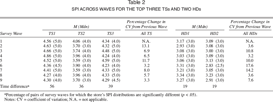
Percentage of pairs of survey waves for which the store's SPI distributions are significantly different (p < .05).

Notes: CV = coefficient of variation; N.A. = not applicable.

As we have discussed, we consider the prices (and, for the TSs, feature promotions) of 49 product categories identified by GfK. To determine the category importance by store format, we calculate, for each household that shops at a certain format and for each product category, the category's share of total household spending at that format. Within each store type, these shares of wallet strongly differ among categories and, for a given category, among house-holds. Out of the 49 product categories considered, the 9 categories with the highest spending overall (Meat, Alcoholic Drinks, Soft Drinks, Vegetables, Fine Meat, Cheese, Fruit, Bread, and Milk & Dairy Drinks) comprise more than half the budget spent at both TS (58.1%) and HD chains (51.7%). Spending shares of individual categories differ markedly between the two store formats. For example, whereas Meat has the highest proportion of the shopping budget at TSs (11.3%), its spending share at HDs is only 3.3%. Conversely, Biscuits & Cookies represent only 3.6% of purchases at TSs but account for 5.1% of HD spending (a list of all categories and their average shares of wallet can be obtained from the first author).

During our observation period, the Dutch retailers were engaging in a price war, which involved price changes for thousands of items spread across multiple categories and comprised multiple rounds that extended beyond our observation period (see, e.g., Van Heerde, Gijsbrechts, and Pauwels 2008). This price war facilitates the assessment of how price changes affect stores’ price images because it was accompanied by some variation in different category prices at the different stores throughout the data period. Table 3 contains descriptive statistics of the weekly category prices by store for the five highest- and lowest-selling categories (the table with all 49 categories can be obtained from the authors). Clearly, prices for a given category vary across chains and, within a given chain, across weeks. We observe the largest over-time variation for Skin Cosmetics, Cleaning, and Bake & Dessert items, while prices are most stable for Oils & Fats, Biscuits & Cookies, and Salted Snacks.

Table 3

Category Price (And Feature) Descriptives For The Top Three Tss And Two Hds

		Price												Feature^a
		M						CV^b						M	CV
Product Category	SOW	TS1	TS2	TS3	HD1	HD2	All	TS1	TS2	TS3	HD1	HD2	All	All TS	All TS
Top Five Share-of-Wallet Categories
Meat	10.03%	1.27	.86	1.14	.68	.67	1.05	.08	.12	.12	.10	.12	.07	.014	.727
Alcoholic Drinks	7.30%	1.30	.80	.87	.85	.81	.95	.08	.16	.18	.20	.31	.12	.012	.927
Vegetables	6.20%	1.21	.91	1.06	.67	.62	.98	.14	.10	.12	.11	.09	.09	.001	1.331
Fine Meat	6.10%	1.28	1.13	1.21	.55	.55	1.11	.07	.10	.10	.12	.14	.08	.005	2.099
Fruit	5.80%	1.25	1.01	1.18	.70	.69	1.05	.17	.15	.14	.14	.17	.10	.008	1.591
Bottom Five Share-of-Wallet Categories
Breakfast Products	.30%	1.05	.95	1.18	.59	.61	1.01	.08	.16	.15	.13	.13	.11	.013	1.278
All-Purpose Cleaners	.30%	1.07	.90	1.03	.28	.59	.90	.23	.23	.31	.75	40	.11	.010	1.302
Cleaning Products	.20%	1.52	.96	1.10	.69	.35	.83	.77	1.18	1.39	.65	49	.26	.000	1.660
Pizza/Snack Food	.20%	1.33	1.03	1.11	1.06	3.41	1.14	.10	.13	.15	.05	.00	.07	.014	.829
Vinegar	.14%	1.43	.99	1.20	.69	.80	1.09	.14	.08	.10	.09	.11	.04	.009	1.745

Percentage of stores in the chain carrying a feature promotion times the percentage of products promoted in that category (available from GfK for TSs only).

For each chain and category, we calculate coefficient of variation as (1) the standard deviation of the category price index across all weeks, divided by (2) the average category price index across these same weeks.

Notes: SOW = share of wallet; CV = coefficient of variation.

To identify the link between actual prices and beliefs, we calculate, for each store, the Spearman rank correlation between the (median) SPI in each wave (across survey respondents for that wave and store) and the overall actual store price index for that wave. The average correlation (across stores) for the unweighted price index is .12 for the TS and .23 for the HD stores, suggesting a positive but weak link between SPI and actual store-level prices.¹¹ Spearman rank correlations between SPIs and specific category prices show wide variation. For TSs, we obtain the highest values for Milk (.21), Cake (.19), and Cheese (.18), while HDs yield the strongest links for Biscuits & Cookies (.07) and Fine Meat (.07). These correlations, however, should be considered with caution because they only rely on variation in specific category prices across the nine survey weeks, which—especially for HDs—is inherently limited. The two rightmost columns of Table 3 summarize the feature support for the store- and week-specific category prices, showing that although this support is limited on average, there is variation across stores and observation weeks.

Instead of calculating the correlation by store and then averaging, we also computed one correlation on the stacked observations of all stores. The results are similar, with a correlation of .214 for TSs and .014 for HDs.

In summary, the data exploration shows that (1) consumers perceive different stores differently with respect to overall expensiveness, (2) price perceptions evolve over time, (3) actual weekly category prices show important variation across both stores and observation weeks, and (4) (category) store prices and SPIs seem to be linked. Yet these rough descriptives do not reveal how SPIs for specific households and stores are updated after a household visit to these stores. Specifically, they only confront the SPI with prices within the survey weeks, ignoring the price signals that households may have encountered in between. Moreover, they do not indicate why some category prices are more influential than others. The results of our model allow us to tap into these questions, but we first discuss how the category characteristics are operationalized.

Category Characteristics

Our goal is to assess the effect of “exogenous” category drivers (similar to, e.g., Bell, Chiang, and Padmanabhan 1999; Bolton 1989; Narasimhan, Neslin, and Sen 1996; Pauwels, Srinivasan, and Franses 2007) on the informativeness of category prices for SPI formation. Thus, our measures of the category drivers do not vary by week or store chain. Making the category drivers store or time specific would not only reduce actionability but also create endogeneity: if we were to operationalize the category drivers (e.g., purchase frequency) by store while estimating common learning parameters across stores, we could overstate the impact of category drivers if stores that differ on these category characteristics (e.g., have higher purchase frequencies) are also better at selecting categories that matter for SPI formation and have the better SPIs. Our market-level measures avoid this problem.¹² Still, because the business models of TSs and HDs are vastly different, we assess the management-related category drivers (i.e., expensiveness, price range, promotion frequency and depth, and number of SKUs) separately for these two types of stores. Moreover, because category purchase frequency and volume may strongly differ between households even within a store type, we assess these two drivers by store format and household. For storability and quality differentiation, which are category characteristics obtained from survey data independent of the store, we use the same measures for both store formats.

Such endogeneity issues are unlikely with our current approach. First, even if stores use price cuts more often in categories that are influential, we do not expect that to be a problem. Our objective is not to assess the overall impact of price changes across categories (which might, indeed, be overestimated if effective categories have more price changes) but rather to explain differences in the impact of prices estimated by category. Our model allows for differential category-price effects (which, given the observed price variation within categories, can be reliably assessed) such that endogeneity from differences in the use of price cuts across categories is less likely to be an issue here. Endogeneity caused by reversed causality is also unlikely: SPIs differ across consumers for a given store, and it is unlikely that retailers adjust their prices to SPIs held by individual consumers (for a similar argument, see Van Heerde, Gijsbrechts, and Pauwels 2008).

To guide the operationalization of the category characteristics, we follow previous cross-category studies in the marketing literature. Table 4 lists all characteristics, along with their median¹³ and standard deviation, for the two store formats. The table reveals substantial variation in the levels of the characteristics—both between store formats and among categories within a format—making them a useful basis for estimation for each of the store types.

Table 4

Category Characteristics: Descriptives

		TSs		HDs
Characteristic	Operaionalization	Mdn	SD	Mdn	SD
Purchase frequency^a	Average number of category purchase occasions per week for the household across all stores (of the format) and weeks in which the household was part of the panel (similar to Fader and Lodish [1990] and Bell, Chiang, and Padmanabhan [1999])	.082	.184	.106	.162
Purchase volume^a	Average number of typical packs bought by the household in the category per category purchase occasion across all stores (of the format) and weeks. A typical pack is the median of the size of one package across all SKU purchases in the category	1.099	.592	1.177	.568
Expensiveness	Average price of a typical pack in the category across all stores (of the format), weeks, and households (similar to, e.g., Fader and Lodish 1990; Narasimhan, Neslin, and Sen 1996; Pauwels, Srinivasan, and Franses 2007)	1.542	.933	1.219	.744
Price range	Regular price difference between the least and the most expensive SKU in the category across stores (of the format) and weeks (similar to, e.g., Briesch et al. 1997; Pauwels, Srinivasan, and Franses 2007; Vanhuele and Drèze 2002)	4.980	17.582	.600	4.260
Promotion depth	Average promotional price cut in the category across stores (in the format) and weeks. We calculate the price cut for a given category, store, and week as a weighted average, across category SKUs, of the percentage difference between regular and promoted price for each promoted SKU (see the next operationalization; for a similar approach, see Fok et al. 2006; Nijs et al. 2001; Raju 1992).	.185	.033	.148	.035
Promotion frequency	For a given category and store (in the format), promotional frequency is the weighted 1 average, across category SKUs, of the number of times weekly SKU prices were more than 5% below the mode prices (“regular prices”) of those SKUs (similar to, e.g., Fok et al. 2006; Nijs et al. 2001; Raju 1992).	6.425	9.809	15.371^c	12.352
Number of SKUs	Number of different SKUs in the category across stores of that format (similar to, e.g., Bell, Chiang, and Padmanabhan 1999; Macέ and Neslin 2004; Pauwels, Srinivasan, and Franses 2007)	1,134	1,553	197	297
Quality differentiation	Using a two-item scale (1 = “strongly disagree,” and 5 = “strongly agree”): “In the product category [X], there are big differences in quality between the various brands (between the shops’ own brands).”^b	3.20	.453	3.20	.453
Storability	Indicator of ability to stockpile (0 = “not storable,” 1 = “storable”), based on expert ratings (similar to, e.g., Bell, Chiang, and Padmanabhan 1999; Macέ and Neslin 2004; Narasimhan, Neslin, and Sen 1996)	0	.487	0	.487

Purchase frequency and purchase volume are store format–, category-, and household-specific variables. For these variables, the rightmost columns report category averages across households.

Survey data collected in the study by Steenkamp et al. (2004). We thank the authors for making the information available.

Note that our promotion frequency measure is relative to the store's assortment size. Absolute numbers are much lower for discounters compared with TSs.

Because some distributions are quite skewed, we focus on the median rather than the mean.

Results

Initial SPI Beliefs

As we outlined previously, we specify consumers’ initial beliefs about a store as a function of nonprice cues. Building on previous literature (e.g., Baker et al. 2002; Hamilton and Chernev 2013), we use available perceptions on (1) store assortment, (2) cleanliness (as a component of store ambiance), (3) advertised promotions, and (4) service (which we obtain as a summated scale of waiting time at the checkout, friendliness, and service of store personnel). Given the ordinal scale of these data (1 = “excellent,” and 9 = “very bad,” after reversing them for consistency with the SPI data), we use ordinal regressions (the CATREG procedure in SPSS) to relate these cues to store price perceptions in the first survey wave (not used for estimation later on), across households and stores in that wave. Table 5 shows the results by store format. As we expected, we obtain a positive association between advertised promotions and price image (Hamilton and Chernev 2013) and a negative link with cleanliness (Büyükkurt 1986). Although favorable assortment perceptions go along with unfavorable price images in both formats (Hamilton and Chernev 2013), the effect fails to reach significance. Like Baker et al. (2002), we do not find a negative link between store service and SPI, possibly because our “service” items are not closely linked with retailer costs. The nonprice cues explain a significant portion of the initial stated price beliefs in both formats, with an R² above 50% and a hit rate well above the random-assignment cutoff. We use the predicted SPIs from these regressions to initialize the mean and variance of the SPIs in the updating equations (for details, see Web Appendix A).

Table 5

Effects Of Nonprice Cues On Initial Spi Beliefs

		TSs		HDs
Variable	Hypothesis	Coefficient	p-Value	Coefficient	p-Value
Perceived cleanliness	–	-.145	.002	-.290	.049
Perceived promotions	+	.556	.000	.606	.000
Perceived assortment	–	-.024	.949	-.155	.787
Perceived service^a	–	.346	.002	.461	.006
R-square		.529		.508
Hit rate		38.5%		36.1%

Summated scale of perceived friendliness, personnel, and waiting time; Cronbach's alpha = .783 (.735) for TSs (HDs).

Model Fit and Validity

Parameter estimation of our learning model is based on a Markov chain Monte Carlo of 100,000 draws, after discarding the first 60,000 draws as burn-in. Visual inspection of the evolution of the parameters’ sampled values indicates that the simulation chains have converged. Hit rates indicate that, in either store format, the model describes the data well—far better than random assignment (33.3% vs. 12.5% [i.e.,2.5 times higher] for TSs and 24.5% vs. 14.3% [i.e.,1.5 times higher] for HDs). To allow for a more refined assessment, we compare the fit of our proposed model with a (quite stringent) benchmark model that, instead of including the separate category drivers, uses household-specific share-of-wallet weighted prices. Moreover, next to in-sample fit, we also assess the performance in two holdout samples: one considering a new set of households in the calibration period and one considering a new survey wave for the households in the estimation sample. For TSs, our proposed model systematically outperforms this benchmark in sample¹⁴ (benchmark model: deviance information criterion [DIC] = 37,666.0; proposed model: DIC = 36,822.0) as well as in both holdouts (benchmark model: predictive log-likelihood [PLL] = −4,322.7 for holdout households and PLL = −844.7 for the holdout wave; proposed model: PLL = −4,320.5 for holdout households and PLL = −844.5 for the holdout wave). For HDs, the comparison is mixed: the benchmark model performs better in sample (benchmark model: DIC = 9,239.1; proposed model: DIC = 11,464.0) but not in terms of predictive fit (benchmark model: PLL = −1,060.7 for holdout households and PLL = −200.2 for the holdout wave; proposed model: PLL = −940.4 for holdout households and PLL = −200.7 for the holdout wave). This finding suggests that even if the coefficients of the category drivers in the HDs are significant (as we discuss subsequently), their explanatory power is not as strong as those for TSs, and thus, the results for the HD chains should be be treated with some caution. All variance inflation factors are below two, indicating absence of collinearity.¹⁵

To account for the lower flexibility of the benchmark model, we consider the deviance information criterion (DIC) measure for the in-sample comparison here. For the holdout samples, we opt for predictive log-likelihoods (PLLs), which are related to marginal likelihoods (see, e.g., Geweke 2005). Note that lower DIC measures and higher PLLs indicate better fit.

The strongest bivariate correlations are those between purchase frequency and promotion frequency (.465) for TSs and between price range and promotion depth (-.515) for HDs. All other correlations are below .500. The determinant of the correlation matrix is .273 for TSs and .299 for HDs.

Drivers of SPI Learning

Table 6 reports the parameter estimates for each of the chain types—that is, the posterior mean values and their 95% posterior intervals (for brevity, we omit the threshold parameters; details can be obtained from the authors). The feature coefficient (r = .41) shows that advertised prices are more influential than nonfeatured ones. Turning to the category drivers, recall that because the dependent variable is the (log of the) precision of the price signals, a positive sign points to a higher effect of category prices on SPI, whereas a negative sign implies a lower impact. Given the double-log specification, the estimates are interpretable as elasticities indicating the relative importance of the category characteristics for SPI learning.¹⁶

Table 6

Parameter Estimates Learning Model

	TSs			HDs
Variable	M	2.5%	97.5%	M	2.5%	97.5%
Intercept	-.951	-1.247	-.605	-.771	-1.274	-.128
Purchase frequency	-.014	-.022	-.006	.038	.019	.055
Purchase volume	.029	.013	.047	.023	-.007	.047
Expensiveness	.110	.093	.130	.058	.026	.093
Price range	-.095	-.106	-.082	-.104	-.134	-.070
Promotion depth	-.383	-.485	-.299	-.795	-1.001	-.587
Promotion frequency	-.052	-.089	-.013	.024	-.026	.073
Number of SKUs	.025	-.006	.053	.255	.179	.321
Quality differentiation	.345	.220	.467	-.008	-.214	.216
Storability	.264	.235	.291	.056	-.013	.138
Feature	.412	.100	.800	—	—	—
Learning heterogeneity (σ_ξ Equation 5)	.537	.531	.543	.675	.662	.690
Error variance	.250	.231	.274	.121	.105	.139

Notes: The table contains posterior mean parameter estimates, along with the 2.5% lower and upper percentiles of their posterior distribution.

An exception is the coefficient of storability, a dummy for which no log-transform is used. This coefficient thus captures the percentage change in the price signal's precision going from a nonstorable to a storable category.

Category drivers of SPI formation

We first discuss the results for TSs, displayed in Table 6. As the table shows, SPIs are more strongly shaped by prices of expensive categories (β = .110, p < .05)¹⁷ that are storable (β = .264, p < .05) and purchased in larger volumes at a time (β = .029, p < .05), in support of the premise that consumers perceive prices in these categories as more important and relevant to monitor. Categories that the household buys frequently (β = -.014, p < .05) do not contribute more strongly to TSs’ overall price image; one explanation for this finding might be that these regularly purchased categories are bought in a more habitual, “routine” fashion. Surprisingly, prices in frequently promoted categories have a lower impact on SPI formation for TSs (β = -.052, p < .05). Similarly, categories typically subject to deep price cuts provide weaker signals of overall supermarket “cheapness” (β = -.383, p < .05). The promotional volatility may render the prices less indicative of the stores’ (stable) overall price positioning or obscure the reference-price standard. The latter may also explain why categories with a wide price range contribute less to SPI formation (β = -.095, p < .05). The number of SKUs does not have a significant effect for TSs (β = .025, p > .10), suggesting that the positive salience effect and the negative price-overload effect cancel each other out. In contrast, categories with more differentiated quality weigh more heavily on supermarkets’ SPI formation (β = .345, p < .05), possibly because consumers purposefully monitor these prices as part of a price–quality trade-off.

Strictly speaking, there are no p-values in Bayesian estimation. We use this shorthand notation to indicate whether the posterior-density interval (reported in Table 6) excludes zero and refer to it as “significant.”

Turning to the results for HDs (see Table 6) we find that although the effect of purchase volume (i.e., number of packs per purchase) is insignificant (β = .023, p > .05), more frequently purchased categories have a stronger impact on SPI formation (β = .038, p < .05). Thus, shoppers at HD chains continue to monitor prices in categories that they often buy, possibly because they are more price sensitive to begin with. Similar to TSs, category expensiveness has a positive coefficient (β = .058, p < .05), while categories with a wider price range contribute less strongly to price image formation (β = -.104, p < .05). In contrast to TSs, categories with more SKUs weigh more heavily on discounters’ overall price beliefs (β = .255, p < .05), whereas quality differentiation does not play a role (β = -.008, p > .10). We must interpret this finding against the PL-dominated nature of the HD offer, in which quality consistency¹⁸ is typically high and large assortments correspond with horizontal differentiation (e.g., different flavors), which may trigger attention without rendering the distribution (and processing) of prices more complicated. Although the coefficient of promotion frequency is insignificant (β = .024, p > .10), price images in the discount format are particularly insensitive to prices in categories with deep price cuts (β = -.795, p < .05), which may be considered at odds with their positioning of everyday low prices.

Because our quality-differentiation driver captures perceived quality differences in the category market-wide (not by store format), differences within the HD chain may be low even for categories that score highly on this driver.

Implications for Practice

Lighthouse Categories

Our finding that category characteristics other than share of wallet moderate the impact of category prices on SPI suggests that by reducing prices in carefully selected categories, retailers can improve store price perceptions while maximally preserving store revenue. Figure 2 plots the categories along two dimensions: their ability to shape SPI (i.e., the posterior mean of the price signal precision), and their sales share (i.e., the amount spent on the category across periods, households, and chains of a specific format, divided by this amount summed over categories). Because these metrics differ by format, we provide a separate plot for TS (Figure 2, Panel A) and HD chains (Figure 2, Panel B).

Figure 2

Category Pricing And Spi: Retailer Sales Implications

The price signal precisions range between .354 and .977 at TSs and between .401 and 1.099 at HD stores, with median values of .610 and .698, respectively.¹⁹ Although we observe a tendency of a positive link between a category's sales share at a store and its SPI signaling power, this link is far from perfect—that is, there are some categories that capture a high portion of sales, but for which learning is not (proportionally) high, and vice versa. These “deviations” are particularly relevant for SPI management. First, changes in the prices of product categories in the bottom-right quadrant of Figure 2, Panels A and B (“Costly Nonsignals”), are to be avoided. Not only are the price signal precisions in these categories among the lowest, their weight in the typical consumer shopping basket is quite high. For TSs, this is the case for fresh items such as Fruit, Vegetables, or Meat. For HDs, Biscuits & Cookies, for example, hurt revenues without boosting SPI.

The means are .622 and .719, respectively. Using a sign test for each of the 1,176 category pairs, we found the posteriors to differ significantly (p < .05) for 1,158 category pairs at discounters and 1,073 pairs at TSs.

Categories situated at the bottom-left quadrant of Figure 2 (e.g., Paper Towels, Sugar, Eggs) are also of little interest for a retailer aiming to convey a favorable SPI. Although price reductions in these small-share categories entail limited revenue losses, their low informativeness makes them less suited for SPI management (“Spoiled Arms”). Conversely, categories in the top-right position (“Costly Signals”) are deemed informative about the store's overall expensiveness, yet because of their large share of sales, they represent a high risk of subsidization for the retailer. This is the case for Alcoholic Drinks and Soft Drinks, which have a high ability to signal SPI but cover more than 5% of consumers’ shopping budget at either store format.

The top-left quadrant comprises the “Lighthouse” categories. They are particularly notable because they have a high potential to shape SPI while constituting only a small portion of the store's sales, thus entailing little subsidization. Although some of them, such as Soup and Skin Cosmetics, are common to both store formats, most Lighthouse categories are format specific. Breakfast Products and Hair Cosmetics, for example, are good candidates for SPI management at TSs, whereas Laundry Detergents and Rice & Pasta serve that purpose at HDs.

To provide a sense of the economic relevance of these findings, we compare the impact of two feature-supported price-cut scenarios on the price image of the leading TS (TS1). In the first scenario, we consider a 15% price cut in a set of Lighthouse categories that, together, account for approximately 11% of the store's sales. In the second scenario, we adopt the same price cut in two Costly Nonsignals categories (Fruit and Vegetables), which also represent 11% of store sales. Using our parameter estimates, and starting from the store's actual prices and image in the initial period, we then compare the average SPI improvement resulting from these two scenarios across 1,000 draws. Whereas price cuts for Costly Nonsignals lead to a small improvement (.03 rating-point drop) in the chain's SPI, reducing the price in the Lighthouse categories leads to an .22 rating-point drop—an extra improvement of .19. We obtain a comparable result for the discount format (i.e., store HD1), in which price cuts in Costly Nonsignal categories hardly affect SPI, and those in Lighthouse categories entail a .17 (extra) rating point improvement. These figures are not unimportant when viewed against the actual observed variation in ratings. Moreover, they may have economically meaningful traffic implications: rough exploration of the link between households’ SPI for a store and their visit frequency to that store suggests that the SPI difference between the two scenarios corresponds to a .6%–.8% increase in number of weekly visits to the chain per household—a nonnegligible figure in an industry in which every customer (visit) is fiercely fought for.

Household Differences

Considering the posterior price signal precisions for each household and category obtained from our TS model (in which the household sample is larger), we find that, although there is much more heterogeneity in learning across categories²⁰ (SD = .158) than across households (SD = .043), household differences do exist. To further explore these differences, we first cluster households according to their responsiveness to category prices. We obtain four segments that differ in the average level of learning and in the categories used for SPI formation. Next, we link the segments to household characteristics through a multinomial logit model. Building on extant studies, we include consumers’ (self-reported) overall quality and price sensitivity, deal proneness, market mavenism, multiple-store shopping, budget pressure, brand loyalty, and household size as possible drivers. Web Appendix B summarizes the results. Households in the largest segment (Segment 2; 44% of the sample) have the lowest learning parameters. These households are medium-sized, quality-oriented, and brand-loyal households, for whom low prices are not key in store choice and market mavenism is low. The second-lowest learners (Segment 1; 36%) exhibit somewhat similar features, except that they are store rather than brand loyal. Households with the highest learning parameters (Segment 3; 11%) are smaller households with low quality orientation, who visit multiple stores and consider themselves market mavens. The second-highest learners (Segment 4; 10%) have quite a different profile: they are large households who tend to purchase all their products in one store and for whom low regular prices (and not price deals) are key in store selection. This group is a particularly noteworthy target for SPI management because they have larger purchase needs and are likely to allocate their entire purchase basket to the store with a favorable price image. Lighthouse categories such as Hair Cosmetics, Dental Care, and Bakery products seem especially influential for these households. Notably, households’ SPI updating does not seem linked to either their budget constraints or their attention to temporary price offers, suggesting that deal proneness and price focus for the formation of overall price beliefs are separate constructs.

We obtain category heterogeneity as the standard deviation of the learning parameters across categories for each household, averaged across households. We obtain household heterogeneity as the standard deviation of the learning parameters across households for each category, averaged across categories.

Discussion, Limitations, and Further Research

Discussion

In this article, we empirically assess how consumers update their beliefs about the overall expensiveness of a store on the basis of actual category prices encountered in that store. We develop and estimate a model of SPI formation over time, in which category prices act as signals for stores’ expensiveness, with a household-specific signal strength that depends on multiple category factors. In this section, we offer several substantive and managerial insights.

Substantive insights

Our findings corroborate previous observations that categories do not influence store price beliefs in proportion to their market share (Desai and Talukdar 2003) and that, in complex settings, factors that facilitate information access, encoding, and integration drive consumer learning (Hoch and Deighton 1989). As such, we provide empirical support for the contention that selective categories can serve as key value indicators for a store's overall price image (Hamilton and Chernev 2013).

Our empirical results highlight category characteristics that make prices more or less influential. We find that price changes in expensive categories entail stronger adjustments in store price beliefs, which is consistent with Desai and Talukdar (2003), who find SPI to be more strongly correlated with prices of high unit-price categories. This finding substantiates the premise that prices of big-ticket items are more salient and deemed more important to monitor (Hamilton and Chernev 2013). Likewise, prices of storable categories and categories bought in large quantities are more influential in the formation of typical supermarket price images, in line with previous findings that consumers react more strongly to price cuts for “long span” products (Desai and Talukdar 2003) that can be stockpiled (Bell, Chiang, and Padmanabhan 1999; Narasimhan, Neslin, and Sen 1996) and for which large savings can be reaped from low prices. Web Appendix C shows that, indeed, categories with a high “conditional” category purchase share (i.e., categories that capture a large portion of trip spending when bought) tend to have a somewhat higher SPI signaling value.

Our results show that frequently purchased items weigh less heavily in the updating of price beliefs for TSs. Although this finding seems at odds with the experimental findings of Desai and Talukdar (2003), it bears similarity to Bell, Chiang, and Padmanabhan's (1999) observation that price drops are less effective in frequently purchased categories. On the one hand, frequent encounters may make prices more prominent and easy to recall; on the other hand, when consumers feel knowledgeable about prices in these often-bought categories, they may purchase in a more habitual fashion and—especially in complex environments—they may be less inclined to monitor subsequent price changes and integrate them into their SPIs (Monroe and Lee 1999). As such, our result fits well with the notion that knowledgeable consumers often learn less from new incoming information (see, e.g., Ackerberg 2001).

Notably, unlike previous studies, we find that consumers are less likely to use prices of categories characterized by frequent or deep promotions to update their overall price beliefs about the store. This may be partly due to our natural setting: promotional price cuts may stand out more in an experimental context but be less prominent when consumers shop for baskets of products in complex price environments such as real-life stores. In addition, the fact that we consider the impact of price changes on consumers’ SPI adjustments over time may explain the difference in results: consumers might have been less inclined to use temporary, “one-shot” price drops as signs that the store is inexpensive in general. To the contrary, the heavy discounting activity might have made consumers wary about proper reference prices or led them to suspect that the store is regularly overpriced (i.e., “discounting the discounts”; Gupta and Cooper 1992)—an issue to be explored in further research.

To the best of our knowledge, we are the first to empirically assess the impact of other characteristics. We find that categories with a wide price range exert a weaker effect on overall store price beliefs, which suggests that the price spread, rather than signaling the presence of low prices (Hamilton and Chernev 2013), may hamper the establishment of a clear price comparison standard for the category against which the store's prices can be evaluated.

Moreover, we are the first to empirically explore the differential role of categories in the formation of TSs’ and HDs’ price image. We find that categories with many SKUs have higher signaling power at HDs, but not at TSs. Whereas large assortment categories may be more salient, the presence of many (differently priced) SKUs may render category-price comparison (across stores with different assortments) more difficult. The latter effect offsets the former at TSs (whose product category offer covers a multitude of differently priced national brands and PLs) but not at HDs (where large assortments include horizontally differentiated, all-PL items with a much simpler price distribution). With regard to quality differentiation, prices of differentiated categories are more influential at TSs but not at HD stores. In such categories, TS shoppers face the full range of quality tiers and may purposefully monitor price as part of a price–quality trade-off.²¹ Hard-discount stores, in contrast, offer only a limited subset of items (i.e., PLs) that have consistent quality even in categories in which the potential for differentiation is high.

This may be because in such categories, consumers’ perceived risk (and, thus, motivation to learn; Szymanowski and Gijsbrechts 2013) is higher. Our survey data indeed reveal a significant correlation of .378 (p < .05) between consumers’ perceived quality differences and perceived risk in the category.

Notably, unlike for TSs, often-purchased categories have higher SPI signaling value for HDs. Being particularly price oriented, HD shoppers may continue to track the prices of these categories despite their already prevalent knowledge—a task facilitated by the lean HD environment. Finally, whereas TSs’ price image is more strongly shaped by the prices of storable items bought in large quantities, these effects are not significant for HDs. This may be due to the lower price variation in these everyday-low-price stores, especially for staple items, which—along with the smaller set of households and stores—may hamper the effects’ significance. As such, absence of these effects for the HD stores should be treated with caution and verified in future studies.

Managerial implications

Our findings offer useful insights for managers. First, we find that although households exhibit some heterogeneity in their degree of learning, product category prices differ in their impact on SPI. Our results identify categories in which price drops are particularly apt at creating a more favorable price image for the store. For retailers, it would be worthwhile to compare the categories’ SPI-signaling power with their traffic-building propensity (Briesch, Chintagunta, and Fox 2009) or promotion responsiveness (e.g., Bell, Chiang, and Padmanabhan 1999; Narasimhan, Neslin, and Sen 1996), as identified in previous literature. We do find some correspondence between the category signaling value for TSs²² and promotion effectiveness or loss leadership reported in previous studies: (1) categories that strongly contribute to a favorable SPI (e.g., Laundry Detergents, Liquid Detergents, Bakery Items, Beer) are among those with high promotion responsiveness (Bell, Chiang, and Padmanabhan 1999) or are loss leaders (Besanko, Dubέ, and Gupta 2005; Pancras, Gauri, and Talukdar 2013); (2) categories with low signaling value (e.g., Yoghurt [Milk Drinks], Butter/Margarine [Oils & Fats], Bread) have been reported in these studies as less promotion responsive, with fewer loss leaders; and (3) products such as Soft Drinks, Hot Drinks, and Ice Cream are situated in the middle. However, these links are far from perfect. Previous research has found that the products for which (promotional) price cuts enhance in-store category sales are not necessarily products that drive store traffic or basket size (Chen et al. 1999); in the same vein, our results indicate that the categories that entice consumers to (temporarily) switch stores or buy more on promotion are not necessarily the ones that shape consumers’ enduring price beliefs about the store.

Hard-discount stores have not (yet) received much attention in this stream of literature.

Moreover, we show that retailers that aim to improve their overall price perception can select categories (1) that contribute favorably to SPI and (2) in which price cuts do not overly hurt revenue. Successful SPI management should focus on Lighthouse categories, which—though they cover only a small portion of sales—exert a strong impact on the store's overall price beliefs. We identify Lighthouse categories for each store format and show that focusing on such categories entails improvements that are economically meaningful.

We also identify categories that are less suitable to create a favorable price image because they have little signaling power (Spoiled Arms) and/or because SPI improvements from price cuts in these categories come at the cost of important revenue losses (Costly [Non]Signals). Many fresh products fall into the latter type. Retailers whose performance is under pressure should thus refrain from using these products for SPI improvement—a recommendation that contradicts conventional practice (e.g., by Wal-Mart; Berk 2010).

Limitations and Further Research

This study has limitations that pave the way for new research. First, although we document the impact of (featured and nonfeatured) prices, other category-specific instruments such as in-store displays, shelf arrangements, and the use of outer packs may influence the formation of SPIs. For lack of data, we could not analyze the effect of changes in such cues, a topic we leave for further study. Second, although we use price salience/perceived importance, ease of comparison, and ease of recall to explain the category-price effects, we do not have separate measures for these constructs. Further research is needed to ascertain the separate role of these process measures. Third, our data include a period of price war, which may have increased consumers’ attention to prices. Because the price war involved a wide range of categories with very different characteristics, we do not expect our estimates of the relative impact of these categories to be biased. Still, it would be useful to replicate our findings in a setting where price competition is less intense. Fourth, our study focuses on category prices as signals of SPI. This focus is consistent with a category management perspective and with the observation that retailers often express their “differential” advantage in terms of specific category offers. Yet prices within a category may differ in their SPI signaling ability. Consumers may use the prices of leading national brands, available in different stores, as anchors to judge the stores’ overall price levels relative to others. Alternatively, storewide PL prices may stand out in the formation of SPIs. To our knowledge, the role of national brand versus PL prices in SPI development has received little attention,²³ and we hope that our study stimulates work in this area. Fifth, a store's price image may depend on the prices of competing stores. A simple way to address this would be to incorporate relative, instead of absolute, price measures into the model (which is likely to yield similar results because the absolute and relative prices are highly correlated²⁴). Separately incorporating category prices of rival retailers in our current model would allow the competitive impact to differ by rival and category but would lead to a high-dimensionality problem with prohibitive computational costs. We leave this challenge for future studies. Relatedly, in gauging the impact of price changes in Lighthouse (as opposed to other) categories on a store's price beliefs, we use a ceteris paribus approach. To the extent that rival chains would react by dropping prices in these Lighthouse categories as well, the SPI implications may become less rosy, and as such, the anticipated benefits from our recommendations should be treated with caution. Sixth, to the extent that retailers have an understanding of categories that drive SPI and are more likely to feature special prices in those categories, our feature variable may be endogenous. We find the link between a store's SPI and its category feature variables to be very weak and mostly insignificant,²⁵ which suggests that this type of endogeneity is not an issue. However, a formal treatment of possible endogeneity is worthwhile to justify this claim. Seventh, although we show that proper category selection substantially contributes to the improvement of store price beliefs and provides a sense for store patronage implications, we do not formally analyze how SPI changes translate into store traffic and spending. Although the impact of price beliefs on store performance is widely recognized, empirical studies that include SPI as a determinant of store choice are rare (for an exception, see Van Heerde, Gijsbrechts, and Pauwels 2008) and do not accommodate the notion that SPIs themselves evolve on the basis of actual prices. Further research could address the mediating role of SPIs for price-induced changes in store traffic and spending.

In a recent article, Lourenço and Gijsbrechts (2013) investigate the impact of national brand introductions on HDs’ price (and quality) images (and share of wallet).

Correlations between the retailer's own category price and its relative price (i.e., own price divided by the average category price across retailers) are .876 on average, with more than 90% of the correlations higher than .7 and virtually all of them significant at p < .01.

The SPI versus category feature support correlations range between –.116 and .384, with a mean of .004. In total, 90% of the correlations lie between –.075 and .150, and fewer than 5% are significant.

References

Ackerberg

Daniel A.

(2001), “Empirically Distinguishing Informative and Prestige Effects of Advertising,” RAND Journal of Economics, 32(2), 316–33.

Alba

Joseph W.

, Broniarczyk

Susan M.

, Shimp

Terence A.

, and Urbany

Joel E.

(1994), “The Influence of Prior Beliefs, Frequency Cues, and Magnitude Cues on Consumers’ Perceptions of Comparative Data,” Journal of Consumer Research, 21(2), 219–35.

Alba

Joseph W.

, Mela

Carl F.

, Shimp

Terence A.

, and Urbany

Joel E.

(1999), “The Effect of Discount Frequency and Depth on Consumer Price Judgments,” Journal of Consumer Research, 26(2), 99–114.

Arnold

Stephen J.

, Oum

Tae H.

, and Tigert

Douglas J.

(1983), “Determinant Attributes in Retail Patronage: Seasonal, Temporal, Regional, and International Comparisons,” Journal of Marketing Research, 20(May), 149–57.

Baker

Julie

, Parasuraman

, Grewal

Dhruv

, and Voss

Glenn B.

(2002), “The Influence of Multiple Store Environment Cues on Perceived Merchandise Value and Patronage Intentions,” Journal of Marketing, 66(April), 120–41.

Bell

David R.

, Chiang

Jeongwen

, and Padmanabhan

(1999), “The Decomposition of Promotional Response: An Empirical Generalization,” Marketing Science, 18(4), 504–526.

Berk

Christina Cheddar

(2010), “Rollback Those Fears About Wal-Mart Prices,” CNBC.com, (April 9), (accessed December 30, 2014), [available at http://www.cnbc.com/id/36317353/Rollback_Those_Fears_About_Wal_Mart_Prices].

Besanko

David

, Dubé

Jean-Pierre

, and Gupta

Sachin

(2005), “Own-Brand and Cross-Brand Retail Pass-Through,” Marketing Science, 24(1), 123–37.

Bolton

Ruth N.

(1989), “The Relationship Between Market Characteristics and Promotional Price Elasticities,” Marketing Science, 8(2), 153–69.

10.

Briesch

Richard A.

, Chintagunta

Pradeep K.

, and Fox

Edward J.

(2009), “How Does Assortment Affect Grocery Store Choice?” Journal of Marketing Research, 46(April), 176–89.

11.

Briesch

Richard A.

, Krishnamurthi

Lakshman

, Mazumdar

Tridib

, and Raj

S.P.

(1997), “A Comparative Analysis of Reference Price Models,” Journal of Consumer Research, 24(2), 202–214.

12.

Bustillo

Miguel

, and Martin

Timothy W.

(2010), “Wal-Mart Bets on Reduction in Prices,” The Wall Street Journal, (April 9), (accessed December 30, 2014), [http://online.wsj.com/article/SB10001424052702304198004575172271682347064.html].

13.

Büyükkurt

B. Kemal

(1986), “Integration of Serially Sampled Price Information: Modeling and Some Findings,” Journal of Consumer Research, 17(3), 357–73.

14.

Chen

Yuxin

, Hess

James D.

, Wilcox

Ronald T.

, and John Zhang

(1999), “Accounting Profits Versus Marketing Profits: A Relevant Metric for Category Management,” Marketing Science, 18(3), 208–229.

15.

Ching

Andrew T.

, Erdem

Tülin

, and Keane

Michael P.

(2013), “Learning Models: An Assessment of Progress, Challenges and New Developments,” Marketing Science, 32(6), 913–38.

16.

DeGroot

Morris H.

(1970), Optimal Statistical Decisions. New York: McGraw-Hill.

17.

Desai

Kalpesh K.

, and Talukdar

Debabrata

(2003), “Relationship Between Product Groups’ Price Perceptions, Shoppers’ Basket Size, and Grocery Stores’ Overall Store Price Image,” Psychology and Marketing, 20(10), 903–933.

18.

Desmet

Pierre

, and Renaudin

Valérie

(1998), “Estimation of Product Category Sales Responsiveness to Allocated Shelf Space,” International Journal of Research in Marketing, 15(5), 443–57.

19.

Dickson

Peter R.

, and Sawyer

Alan G.

(1990), “The Price Knowledge and Search of Supermarket Shoppers,” Journal of Marketing, 54(July), 42–53.

20.

Erdem

Tülin

, and Keane

Michael P.

(1996), “Decision-Making Under Uncertainty: Capturing Dynamic Choice Processes in Turbulent Consumer Goods Markets,” Marketing Science, 15(1), 1–20.

21.

Erdem

Tülin

, and Keane

Michael P.

, and Sun

Baohong

(2008), “A Dynamic Model of Brand Choice When Price and Advertising Signal Product Quality,” Marketing Science, 27(6), 1111–25.

22.

Fader

Peter S.

, and Lodish

Leonard M.

(1990), “A Cross-Category Analysis of Category Structure and Promotional Activity for Grocery Products,” Journal of Marketing, 54(October), 52–65.

23.

Feichtinger

Gustav

, Luhmer

Alfred

, and Sorger

Gerhard

(1988), “Optimal Price and Advertising Policy for a Convenience Goods Retailer,” Marketing Science, 7(2), 187–201.

24.

Fok

Dennis

, Horváth

Csilla

, Paap

Richard

, and Franses

Philip Hans

(2006), “A Hierarchical Bayes Error Correction Model to Explain Dynamic Effects of Price Changes,” Journal of Marketing Research, 43(August), 443–61.

25.

Gauri

Dinesh K.

, Sudhir

, and Talukdar

Debabrata

(2008), “The Temporal and Spatial Dimensions of Price Search: Insights from Matching Household Survey and Purchase Data,” Journal of Marketing Research, 45(April), 226–40.

26.

Geweke

John

(2005), Contemporary Bayesian Econometrics and Statistics. Hoboken, NJ: Wiley-Interscience.

27.

Gijsbrechts

Els

, Campo

Katia

, and Nisol

Patricia

(2008), “Beyond Promotion-Based Store Switching: Antecedents and Patterns of Systematic Multiple-Store Shopping,” International Journal of Research in Marketing, 25(1), 5–21.

28.

Grewal

Dhruv

, and Levy

Michael

(2007), “Retailing Research: Past, Present, and Future,” Journal of Retailing, 83(4), 447–64.

29.

Gupta

Sunil

, and Cooper

Lee G.

(1992), “The Discounting of Discounts and Promotion Thresholds,” Journal of Consumer Research, 19(3), 401–411.

30.

Hamilton

Ryan

, and Chernev

Alexander

(2013), “Low Prices Are Just the Beginning: Price Image in Retail Management,” Journal of Marketing, 77(November), 1–20.

31.

Hoch

Stephen J.

, and Deighton

John

(1989), “Managing What Consumers Learn from Experience,” Journal of Marketing, 53(April), 1–20.

32.

Jensen

Birger Boutrup

, and Grunert

Klaus G.

(2014), “Price Knowledge During Grocery Shopping: What We Learn and What We Forget,” Journal of Retailing, 90(3), 332–46.

33.

Kardes

Frank R.

(1994), “Consumer Judgment and Decision Processes,” in Handbook of Social Cognition, Vol. 2, Robert

S. Wyer

, and Srull

Thomas K.

, eds. Hillsdale, NJ: Lawrence Erlbaum Associates.

34.

Kopalle

Praveen K.

, Mela

Carl F.

, and Marsh

Lawrence

(1999), “The Dynamic Effect of Discounting on Sales: Empirical Analysis and Normative Pricing Implications,” Marketing Science, 18(3), 317–32.

35.

Krider

Robert E.

, and Weinberg

Charles B.

(2000), “Product Perishability and Multistore Grocery Shopping,” Journal of Retailing and Consumer Services, 7(1), 1–18.

36.

Lagorce

Aude

(2009), “Carrefour Pushes Hard to Restore Its Price Image,” MarketWatch.com, (June 30), (accessed December 30, 2014), [available at http://www.marketwatch.com/story/carrefour-detemined-to-restore-price-image].

37.

Lalwani

Ashok K.

, and Monroe

Kent B.

(2005), “A Reexamination of Frequency-Depth Effects in Consumer Price Judgments,” Journal of Consumer Research, 32(3), 480–85.

38.

Lourenço

Carlos J.S.

, and Gijsbrechts

Els

(2013), “The Impact of National Brand Introductions on Hard-Discounter Image and Share-of-Wallet,” International Journal of Research in Marketing, 30(4), 368–82.

39.

Lynch

John G.

, and Ariely

Dan

(2000), “Wine Online: Search Costs Affect Competition on Price, Quality, and Distribution,” Marketing Science, 19(1), 83–103.

40.

Macé

Sandrine

, and Neslin

Scott A.

(2004), “The Determinants of Pre- and Postpromotion Dips in Sales of Frequently Purchased Goods,” Journal of Marketing Research, 41(August), 339–50.

41.

Mägi

Anne W.

, and Julander

Claes-Robert

(2005), “Consumers’ Store-Level Price Knowledge: Why Are Some Consumers More Knowledgeable Than Others?” Journal of Retailing, 81(4), 319–29.

42.

Mazumdar

Tridib

, and Monroe

Kent B.

(1990), “The Effects of Buyers’ Intentions to Learn Price Information on Price Encoding,” Journal of Retailing, 66(1), 15–32.

43.

Mazumdar

Tridib

, Raj

S.P.

, and Sinha

Indrajit

(2005), “Reference Price Research: Review and Propositions,” Journal of Marketing, 69(October), 84–102.

44.

Mela

Carl F.

, Gupta

Sunil

, and Lehmann

Donald R.

(1997), “The Long-Term Impact of Promotions and Advertising on Consumer Brand Choice,” Journal of Marketing Resesearch, 34(May), 248–61.

45.

Mela

Carl F.

, Jedidi

Kamel

, and Bowman

Douglas

(1998), “The Long-Term Impact of Promotions on Consumer Stockpiling,” Journal of Marketing Research, 35(May), 250–62.

46.

Miyazaki

Anthony D.

, Sprott

David E.

, and Manning

Kenneth C.

(2000), “Unit Prices on Retail Shelf Labels: An Assessment of Information Prominence,” Journal of Retailing, 76(1), 93–112.

47.

Monroe

Kent B.

, and Lee

Angela Y.

(1999), “Remembering Versus Knowing: Issues in Buyers’ Processing of Price Information,” Journal of the Academy of Marketing Science, 27(2), 207–225.

48.

Narasimhan

Chakravarthi

, Neslin

Scott A.

, and Sen

Subrata K.

(1996), “Promotional Elasticities and Category Characteristics,” Journal of Marketing, 60(April), 17–30.

49.

Nielsen

A.C.

(2004), “Survey of Trade Promotion Practices,” technical report.

50.

Nielsen

A.C.

(2008), “Grocery Store Choice and Value for Money: A Global Nielsen Consumer Report,” technical report, January.

51.

Nijs

Vincent R.

, Dekimpe

Marnik G.

, Steenkamp

Jan-Benedict E.M.

, and Hanssens

Dominique M.

(2001), “The Category-Demand Effects of Price Promotions,” Marketing Science, 20(1), 1–22.

52.

Nyström

Harry

(1970), “Retailing Pricing: An Integrated Economic and Psychological Approach,” doctoral thesis, Economic Research Institute, Stockholm School of Economics.

53.

Pancras

Joseph

, Gauri

Dinesh K.

, and Talukdar

Debabrata

(2013), “Loss Leaders and Cross-Category Retailer Pass-Through: A Bayesian Multilevel Analysis,” Journal of Retailing, 89(2), 140–57.

54.

Pauwels

Koen

, Srinivasan

Shuba

, and Franses

Philip Hans

(2007), “When Do Price Thresholds Matter in Retail Markets?” Marketing Science, 26(1), 83–100.

55.

Planet Retail (2014), “Western European Trends, 2014: Retail Trends and Forecasts,” report, (June).

56.

Progressive Grocer (2007), “Category Management Goes Beyond Grocery: Cannondale Report,” technical report, (February).

57.

Raju

Jagmohan S.

(1992), “The Effect of Price Promotions on Variability in Product Category Sales,” Marketing Science, 11(3), 207–220.

58.

Shin

Sangwoo

, Misra

Sanjog

, and Horsky

Dan

(2012), “Disentangling Preferences and Learning in Brand Choice Models,” Marketing Science, 31(1), 115–37.

59.

Steenkamp

Jan-Benedict E.M.

, Geyskens

Inge

, Gielens

Katrijn

, and Koll

Oliver

(2004), “A Global Study into Drivers of PL Success,” report, AIM, Brussels.

60.

Steenkamp

Jan-Benedict E.M.

, and Kumar

(2009), “Don't Be Undersold!” Harvard Business Review, 87(December), 90–95.

61.

Steenkamp

Jan-Benedict E.M.

, van Heerde

Harald

, and Geyskens

Inge

(2010), “What Makes Consumers Willing to Pay a Price Premium for National Brands Over Private Labels?” Journal of Marketing Research, 47(December), 1011–24.

62.

Szymanowski

Maciej

, and Gijsbrechts

Els

(2013), “Patterns in Consumption-Based Quality Learning for Consumer Packaged Goods,” International Journal of Research in Marketing, 30(3), 219–35.

63.

Urbany

Joel E.

, Dickson

Peter R.

, and Kalapurakal

Rosemary

(1996), “Price Search in the Retail Grocery Market,” Journal of Marketing, 60(April), 91–104.

64.

Van Heerde

Harald

, Gijsbrechts

Els

, and Pauwels

Koen

(2008), “Winners and Losers in a Major Price War,” Journal of Marketing Research, 45(October), 117–28.

65.

Van Heerde

Harald

, Mela

Carl F.

, and Manchanda

Puneet

(2004), “The Dynamic Effect of Innovation on Market Structure,” Journal of Marketing Research, 41(May), 166–83.

66.

Vanhuele

Marc

, and Drèze

Xavier

(2002), “Measuring the Price Knowledge Shoppers Bring to the Store,” Journal of Marketing, 66(October), 72–85.

67.

Wakefield

Kirk L.

, and Jeffrey Inman

(1993), “Who Are the Price Vigilantes? An Investigation of Differentiating Characteristics Influencing Price Information Processing,” Journal of Retailing, 69(2), 216–33.

68.

Zeithaml

Valarie A.

(1988), “Consumer Perceptions of Price, Quality, and Value: A Means-End Model and Synthesis of Evidence,” Journal of Marketing, 52(July), 2–22.

69.

Zielke

Stephan

(2010), “How Price Image Dimensions Influence Shopping Intentions for Different Store Formats,” European Journal of Marketing, 44(6), 748–70.

Supplementary Material

Please find the following supplemental material available below.

For Open Access articles published under a Creative Commons License, all supplemental material carries the same license as the article it is associated with.

For non-Open Access articles published, all supplemental material carries a non-exclusive license, and permission requests for re-use of supplemental material or any part of supplemental material shall be sent directly to the copyright owner as specified in the copyright notice associated with the article.

0.13 MB

0.00 MB