
Abstract
The purpose of this study is to investigate a functional relation between item exposure parameters (IEPs) and item parameters (IPs) over parallel pools. This functional relation is approximated by a well-known tool in machine learning. Let P and Q be parallel item pools and suppose IEPs for P have been obtained via a Sympson and Hetter–type simulation. Based on these simulated parameters, a functional relation k = fP (a, b, c) relating IPs to IEPs of P is obtained by an artificial neural network and used to estimate IEPs of Q without tedious simulation. Extensive experiments using real and synthetic pools showed that this approach worked pretty well for many variants of the Sympson and Hetter procedure. It worked excellently for the conditional Stocking and Lewis multinomial selection procedure and the Chen and Lei item exposure and test overlap control procedure. This study provides the first step in an alternative means to estimate IEPs without iterative simulation.
Keywords
Introduction
Computerized adaptive testing (CAT) has proved to be an effective electronic testing mechanism for many real-world test practices. Each year, the CAT version of the armed services vocational aptitude battery (CAT-ASVAB) is administered to hundreds of thousands of applicants entering or advancing their careers in the military services. Using item response theory, CAT adapts test items to a test-taker’s estimated ability and may shorten the test length without losing assessment precision. CAT is emerging as a useful alternative to the conventional paper-and-pencil group-administered testing.
One practical advantage of computerized adaptive tests is that they can be administered on a flexible schedule rather than at fixed times. The convenience and flexibility for examinees, however, may severely compromise test security if item exposure is not well controlled. Chang and Ansley (2003) gave a comparative study of various item exposure control methods used in CAT. To date, randomized item selection (e.g., McBride & Martin, 1983) and conditioned item selection (e.g., Sympson & Hetter, 1985) are main approaches used to avoid item overexposure in CAT (Way, 1998). Although randomized item selection is simple and easy to implement, this approach does not control item exposure well but shuffles items (Sympson & Hetter, 1985). On the other hand, conditioned item selection can control item exposure well so that most items are administered with exposure rates less than a prespecified maximum item exposure rate.
The procedure of conditioned item selection was originally proposed by Sympson and Hetter (SH) in 1985 and served as a foundation for other conditioned item selection methods. Because of the high-stakes nature of the test results, CAT-ASVAB has been administered with item exposure control based on the SH procedure (Hetter & Sympson, 1997; Segall & Moreno, 1999). The SH procedure was designed to directly control item exposure in a probabilistic fashion. Three kinds of probability are defined in this approach: P(S), the probability that an item is selected as the best item based on a CAT algorithm; P(A), the probability that an item is actually administered to examinees; and P(A|S), the conditional probability that an item is administered, given that it is selected as the best item, also named item exposure parameter (IEP). Because an item must be selected first before it can be administered, the relationship among these three probabilities becomes P(A) = P(A|S) × P(S). To meet the requirement that no item has been administered more often than a prespecified maximum item exposure rate r max, the condition thus becomes P(A|S) × P(S) ≤ r max.
Although it is simple to decide P(A|S) as long as P(S) is known, determining P(S) is not trivial. Furthermore, when P(A|S) for an item is decided, the P(S) values for the rest of the items in the pool will be changed, as will the P(A|S) values associated with them. Thus, a series of CAT simulation is needed to find stabilized P(S) values and P(A|S) values under which all P(A) values are less than or equal to r max. The procedure for conducting iterative simulation is described later in the article.
Way (1998) observed that probabilistic item exposure control such as the SH procedure may not be adequate to guarantee a secure CAT implementation and suggested a system of rotating item pools to prevent a security breach. These pools should have similar distribution of contents and statistical attributes to support uniform measurement quality to examinees. Using techniques of constrained combinatorial optimization, Ariel, Veldkamp, and van der Linden (2004) have established a procedure to construct rotating item pools. These pools have identical distribution of item parameters (IPs) and thus are parallel pools constructed from a master pool. Because the SH-type IEPs cannot be solved analytically (van der Linden, 2003), finding a mechanism to estimate IEPs of parallel pools without tedious simulation becomes a challenging and interesting research problem.
Purpose of the Study
Today, most SH-type procedures find IEPs by iterative simulation of CATs. Although these parameters cannot be solved analytically (van der Linden, 2003), this does not mean that they cannot be estimated without tedious simulation. The purpose of this study is to investigate a functional relation between IEPs and IPs over parallel pools. This functional relation is approximated by a knowledge-based tool in machine learning. Because rotating parallel pools are useful in CAT implementations, it is suitable to restrain this study to parallel pools. Let P and Q be parallel item pools and suppose IEPs of P have been found via conventional SH-type simulations. Based on these simulated IEPs, a functional relation k = fP (a, b, c) relating IPs to IEPs of the pool P is approximated by an artificial neural network (ANN) and used to estimate IEPs of Q without tedious simulation.
The original Sympson and Hetter (1985) procedure uses the maximal item information criterion to select items and adjusts IEPs in successive iterations with a well-known formula. Later variants of the SH procedure modify either the item selection criterion or the IEP updating formula to achieve more robust results. This study examined many popular extensions of the SH procedure. Various item exposure controls based on the SH procedure will be discussed next, which is followed by an introduction to the tools used in this study, particularly the ANN from machine learning. Then, item pools will be introduced with an operational definition of parallel pools. Simulation studies and results will follow the description of item pools. A discussion of the results and possible future studies will close this article.
Item Exposure Control
Item exposure control in tests is needed to maintain test security in practical CATs. The popular SH procedure and its many variants used in this study are described in the following. These are the primary procedures adopted in today’s CAT implementation or research studies regarding item exposure control.
The Sympson and Hetter (1985) Procedure
An item response model, which specifies how likely an examinee will answer an item
correctly depending on a few characteristics of the item and the latent ability of
the examinee, must be specified first. This study used the three-parameter logistic
item response model (3PLM), in which the probability of a correct response given an
ability level  where ai
is the item discrimination parameter, bi
is the item difficulty parameter, and ci
is the pseudo-guessing parameter of item i. The Sympson and Hetter (1985)
procedure uses the maximal item information criterion to select items. A selected
item is administered when a uniform random number is smaller than the IEP of that
item. If the item is not administered, it is removed from the pool for the remaining
test of a test-taker and the item with the next best item information is selected for
administration consideration. An unbiased value of zero was assumed as the initial
ability estimate for a test-taker, and the expected a posterior (EAP) estimation was
used to estimate the latent ability after an item was administered.
where ai
is the item discrimination parameter, bi
is the item difficulty parameter, and ci
is the pseudo-guessing parameter of item i. The Sympson and Hetter (1985)
procedure uses the maximal item information criterion to select items. A selected
item is administered when a uniform random number is smaller than the IEP of that
item. If the item is not administered, it is removed from the pool for the remaining
test of a test-taker and the item with the next best item information is selected for
administration consideration. An unbiased value of zero was assumed as the initial
ability estimate for a test-taker, and the expected a posterior (EAP) estimation was
used to estimate the latent ability after an item was administered.
After a target r
max is set and assuming an initial value of 1.0 for the IEP
k of all items, a series of CAT simulation is conducted to a
population of simulees. An iteration of simulation consists of a complete run of CATs
to all simulees of interest according to the CAT algorithm specified above. At the
end of each iteration, P(S) and P(A) are determined
for each item by computing the proportion of times an item has been selected and
administered, respectively. The maximum value of P(A) in the item
pool is noted and k is redefined for each item as follows:
 To guarantee that a test-taker will take a complete test before
exhausting the item pool, the l largest IEPs are set to 1.0 where
l is the test length. The iterative simulation is repeated until
all ks are stabilized and the maximum value of P(A)
is slightly above r
max and oscillates in successive simulations.
To guarantee that a test-taker will take a complete test before
exhausting the item pool, the l largest IEPs are set to 1.0 where
l is the test length. The iterative simulation is repeated until
all ks are stabilized and the maximum value of P(A)
is slightly above r
max and oscillates in successive simulations.
The van der Linden (2003) Alternatives
After analyzing formal properties of the SH procedure, van der Linden pointed out
that the SH procedure has a couple of unpleasant features: it is generally
time-consuming and it can show unexpected behavior of exposure rates for some items
at some steps and may have difficulty converging to a stable state at all (van der Linden, 2003). The
researcher proposed a few alternative formulas in the IEP updating step to achieve
more effective results. Some alternatives proposed by van der Linden have shown quite
effective improvements over the SH procedure. Among them, Formula 12, recommended by
the author, was considered in this study. This formula defines the IEP updating step
as follows:
 where 0 ≤ γ ≤ r
max∕P
(t)(A) is an adjustable parameter and
the superscript indicates the iteration number. A few special features about this
formula can be noted: (a) the adjusting criterion is based on the observed exposure
rate P(A); and (b) when the observed exposure rate of an item is
below the target, its IEP is not adjusted. Experiments have shown that with this new
formula, the maximum observed exposure rate decreases steadily with the number of
iterations, and IEPs converge to a stable state faster than the SH procedure.
where 0 ≤ γ ≤ r
max∕P
(t)(A) is an adjustable parameter and
the superscript indicates the iteration number. A few special features about this
formula can be noted: (a) the adjusting criterion is based on the observed exposure
rate P(A); and (b) when the observed exposure rate of an item is
below the target, its IEP is not adjusted. Experiments have shown that with this new
formula, the maximum observed exposure rate decreases steadily with the number of
iterations, and IEPs converge to a stable state faster than the SH procedure.
The Stocking and Lewis (1998, 2000) Multinomial Procedure
The SH procedure is not flawless. Stocking (1994) pointed out that this procedure may not converge during
its simulation stage. Instead of setting the highest IEPs back to 1.0 in the fix-up
step of the SH procedure, Stocking and Lewis (1998, 2000) proposed a more robust multinomial
model to select items. In the basic unconditional model of their approach, a list of
items ordered from the highest item information to the lowest item information
together with the IEPs ki
is formed. New probabilities li
= (1 − k
1)*…*(1 − ki
−1)*ki
are computed and normalized to form a multinomial distribution from which
an item is selected for administration consideration. A proper length for the list is
approximated by the ratio of the pool size and the test length. The unconditional
multinomial model conducts iterative simulation to a population of simulees with a
special distribution of abilities. However, the more advanced conditional Stocking
and Lewis procedure conducts iterative simulation conditional on ability. The ability
scale is first discretized into M levels:
The Chen and Lei (2005) Item Exposure and Test Overlap Control
Test security can be considered from two levels: item exposure and test overlap. Item
exposure controls the exposure rate of individual items, whereas test overlap is
concerned with how similar two examinees receive the test on average. Davey and Parshall (1995)
proposed an item selection mechanism conditional on items administered earlier in a
test to solve the test overlap issue. The Davey and Parshall procedure is
time-consuming and may be difficult to implement in a practical test environment
(Stocking & Lewis,
1998). Using a relationship between the test overlap rate and the variance
of observed exposure rates, Chen
and Lei (2005) developed a modified SH procedure to control item exposure
and test overlap at the same time. In their approach, given a desired test overlap
rate T
0, the corresponding variance 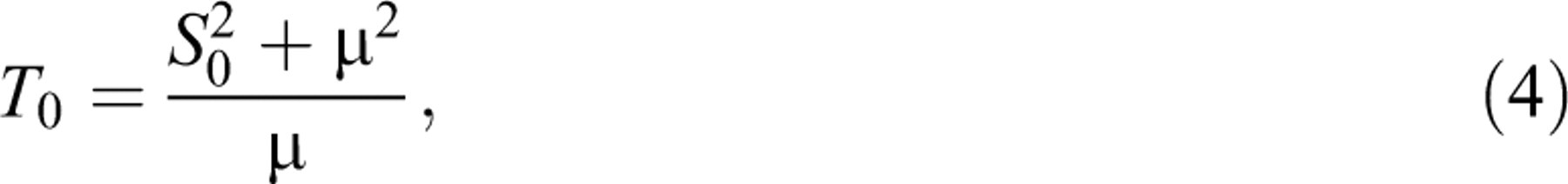 where μ is equal to the test length divided by the pool size. Let
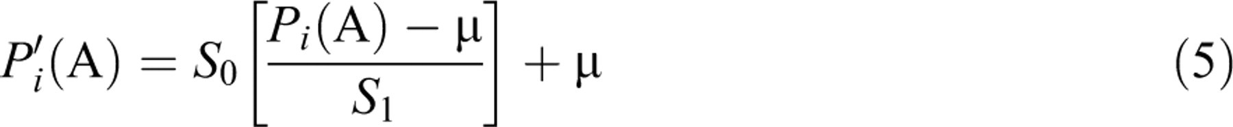 Then, the updated IEP
  The iterative simulation will be monitored from two perspectives: the
maximum observed exposure rate and the test overlap rate. When these two indices
stabilize and are close to the target r
max and T
0, the iteration stops and simulated IEPs can be used to control exposure
at both the item and test levels (Chen & Lei, 2005).
The iterative simulation will be monitored from two perspectives: the
maximum observed exposure rate and the test overlap rate. When these two indices
stabilize and are close to the target r
max and T
0, the iteration stops and simulated IEPs can be used to control exposure
at both the item and test levels (Chen & Lei, 2005).
A Structural Requirement for Tests—the Content-Balancing Requirement
A test may need to explore an examinee’s ability in different content areas of a subject at the same time. Content balancing can be added as a structural constraint to a CAT implementation. Items from different content areas must be administered in a preset manner such that the content coverage is balanced (Leung, Chang, & Hau, 2003). The original SH procedure can be modified to handle this content-balancing requirement. To do so, one must design a mechanism to select a content area before an item is selected from that area. For example, the content area may be chosen randomly or sequentially. The other approach is to choose the area farthest from its preset coverage requirement (Kingsbury & Zara, 1989).
The Chang and Ying (1999) Stratification Procedure
Item exposure control can be inspected from two alternative perspectives: item overexposure and item underexposure. Overexposed items result in test security problems, whereas underexposed items waste the resources devoted to develop the test items. It has been found that in a 3PLM environment, items with high discrimination parameter are frequently overexposed whereas items with low discrimination parameter are less selected for administration. To overcome this exposure imbalance problem, Chang and Ying (1999) proposed an a-stratified multistage CAT procedure, where items were stratified into a number of levels based on the discrimination parameter. The researchers found that with these stratified procedures, CAT operations were efficient and well balanced with respect to item usage. The SH procedure can be added to deal with item overexposure in the stratified multistage procedure.
Method
Approximating a functional relation between IEPs and IPs is considered a regression problem in statistics. Multiple linear regression (MLR) is commonly used to investigate a linear relationship between independent and dependent variables. However, it will be shown that MLR is not good enough to estimate IEPs from IPs. More delicate regression techniques from other fields must be considered.
ANN for Function Approximation
ANN has been successfully applied to solve many function approximation problems in engineering and social sciences. An ANN simulates the neural system of a brain to learn patterns from examples and uses the learned knowledge to make predictions for future data (Gupta, Jin, & Homma, 2003). A basic data processing unit in a neural net is called a neuron, which is connected to other neurons via synapses. The structure of an ANN refers to the number of neurons and the way they are distributed and connected. To simplify the computation, neurons are scattered into layers and information is transferred from layer to layer. Figure 1 shows the structure of a typical two-layer feed-forward neural net. The input layer represents the independent variables in a function approximation problem, for example, neurons for the IPs a, b, and c. The output layer corresponds to the dependent variables, for example, a neuron for the IEP k in Figure 1. Layers between the input and output layers are called hidden layers. An ANN with hidden layers is also called a multilayer perceptron (MLP). Without a hidden layer, a simple perceptron can hardly learn any interesting functions in practical applications (Minsky & Papert, 1969). Although the neural system of a real brain may not be arranged in such a layer style, it has been shown that an MLP can approximate arbitrarily well any continuous decision region provided that there are enough layers and neurons (Gallant & White, 1992).
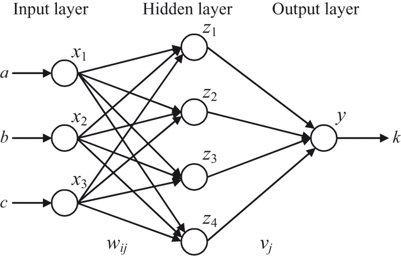
Schema for a two-layer feed-forward artificial neural network.
Each connection between two neurons (i.e., a synapse) has a weight to be learned from
training examples. In a feed-forward network, data flow from the input layer to the
hidden layers and to the output layer in one direction. A hidden layer works like an
intermediate information store that aggregates data from the previous layer. Data
computation at a neuron consist of a weighted averaging step followed by an
activation step
Using ANN to solve a function approximation problem is a two-phase procedure: the
training phase and the operational phase. In the training phase (i.e., the knowledge
acquiring phase), examples with known input-output pairs are used to adjust the
synaptic weights so that computed outputs from the network are as close as possible
to the target outputs. This is commonly done with a so-called back-propagation
technique as follows. Let (a, b, c, t) be a training example in
Figure 1 with (a,
b, c) denoting the IPs of an item and t denoting the
simulated IEP. Therefore, t is the target output for the input
(a, b, c). For the explanation of the back-propagation technique,
notations are modified as follows: the input layer is denoted by
xi
, that is, x
1 = a, x
2 = b, x
3 = c, the hidden layer is denoted by
zj
, that is, 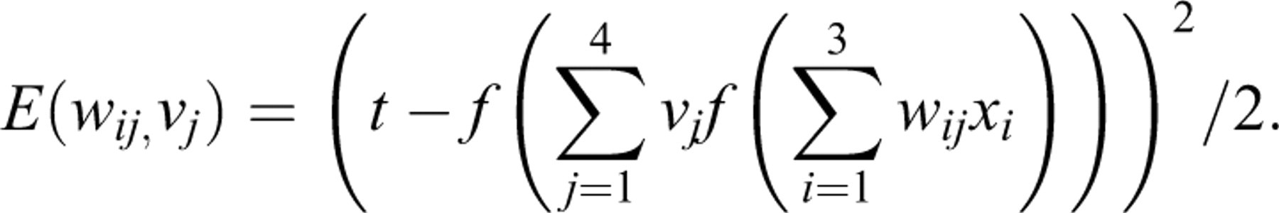
Although this is a complex composite function, using the steepest descent method a
simple formula for the weight adjustment can be derived. The steepest descent method
adjusts the current weight by a multiple of the gradient direction
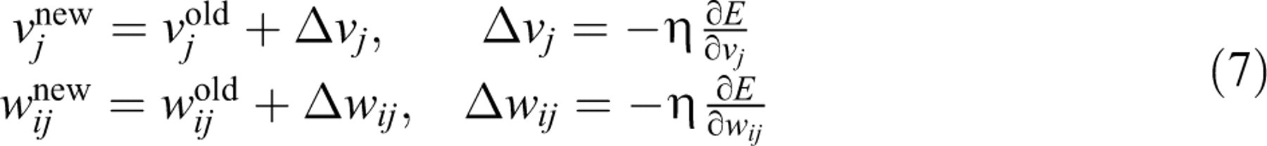 where η is the learning rate. With the chain rule of calculus and a
special feature of the sigmoid function, f′(s) =
f(s)(1 −
f(s)), the weight adjustment can be summarized as
Δvj
= η(t − y) y (1 −
y)zj
and Δwij
= η(t − y) y (1 −
y) zj
(1 − zj
)vjxi
. For a general multilayer neural network with multiple dependent variables,
the weight adjustment is conducted backward from the output layer to the input layer
using the formula
where η is the learning rate. With the chain rule of calculus and a
special feature of the sigmoid function, f′(s) =
f(s)(1 −
f(s)), the weight adjustment can be summarized as
Δvj
= η(t − y) y (1 −
y)zj
and Δwij
= η(t − y) y (1 −
y) zj
(1 − zj
)vjxi
. For a general multilayer neural network with multiple dependent variables,
the weight adjustment is conducted backward from the output layer to the input layer
using the formula 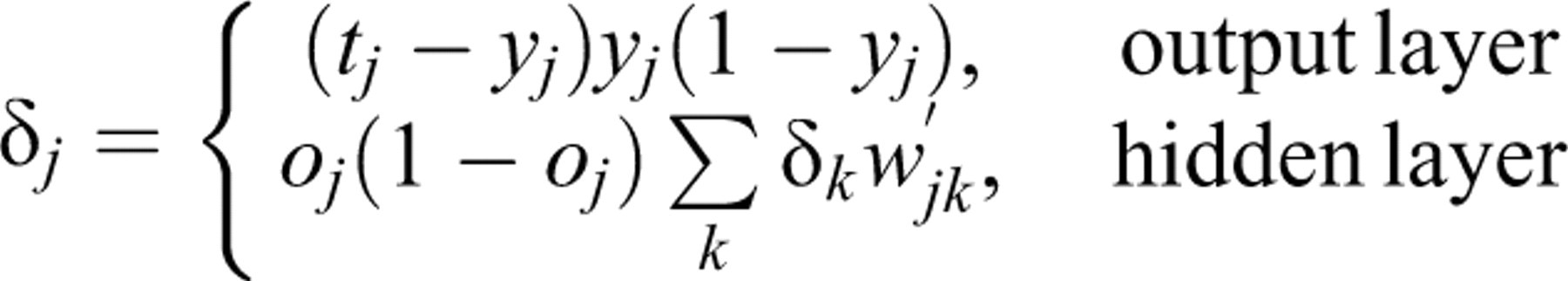 In the above formula, yj
denotes the network output of a dependent variable and
tj
is the corresponding target output. When neuron j is in a
hidden layer, the summation
In the above formula, yj
denotes the network output of a dependent variable and
tj
is the corresponding target output. When neuron j is in a
hidden layer, the summation
During the training phase, network weights are initialized by random numbers first. Then, training examples are sequentially or randomly fed into the network to adjust weights using Equation 7. An epoch of network training is one complete presentation of the training examples to the network. After the network has been trained satisfactorily, it enters the operational phase. Using the trained weights, data with inputs only can be fed into the network to compute outputs. Although the training phase may take some time to obtain satisfactory synaptic weights, the operational phase is usually fast. For example, it took a trained MLP only seconds to compute all IEPs of a pool.
The Proposed Knowledge-Based Approach for Item Exposure Control
First, the input-output pairs of data (ai, bi, ci, ki ), i = 1, …, N = pool size, must be prepared with an SH-type procedure for a training pool, say P. Thus, target IEP ki is obtained from a series of CAT simulation. These data constitute the training examples for an MLP to learn a functional relation k = fP (a, b, c), which is then used to estimate IEPs of parallel pools.
Baringhaus and Franz (2004) Multivariate Two-Sample Test
Parallelism between two item pools will be defined in terms of sample distribution of IPs in the pools. To perform a multivariate two-sample test, a test statistics from Baringhaus and Franz (2004) was adopted. Using the difference of the sum of all the Euclidean interpoint distances between random variables from the two different samples and one-half of the two corresponding sums of distances of the variables within the same sample, Baringhaus and Franz found that this new test provided power similar to that of the Hotelling’s T 2-test under the assumption of normal distributions. In addition, the test also performed well in a distribution-free environment. The Baringhaus and Franz test can be implemented with the cramer package under the free R software environment for statistical computing.
Taylor and Thompson (1986) Random Data Generator
In addition to real parallel pools obtained from an operational CAT, parallel pools
will also be synthesized. To achieve this goal, a random data generator based on a
set of samples must be developed. Taylor and Thompson (1986) have developed such a generator as
follows: First, a multivariate observation xj
is randomly chosen from the given sample set; The nearest m neighbors of xj
from the sample set are determined: xj1
, …, xjm
. The mean Random samples u
1, …, um
are generated using uniform distribution on the interval
(
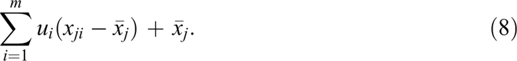 The above procedure can be repeated as many times as needed to provide
enough random data. The Taylor
and Thompson (1986) procedure is implemented as a subroutine in the
International Mathematics and Statistics Library (IMSL) numerical libraries.
The above procedure can be repeated as many times as needed to provide
enough random data. The Taylor
and Thompson (1986) procedure is implemented as a subroutine in the
International Mathematics and Statistics Library (IMSL) numerical libraries.
Item Pools
Seven item pools were used in this study with 360 items in each pool. Descriptive statistics of the IPs for each pool are shown in Table 1. The first three pools (training, T1, T2) consisted of IPs actually calibrated from multiple forms of a large-scale standardized test based on 3PLM. They were assembled from a large master pool by requiring similar statistical attributes in each pool. Although previous studies on parallel pools did not give an explicit definition for the concept, they all emphasized on similar statistical attributes to support parallelism between pools (Ariel, Veldkamp, & van der Linden, 2004; Way, 1998). Thus, an operational definition for parallel pools in this study is given as follows.
Descriptive Statistics of Item Parameters for Pools Used in the Study
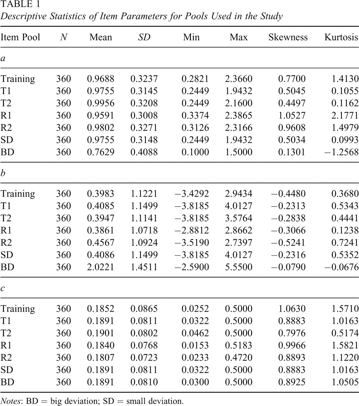
Notes: BD = big deviation; SD = small deviation.
Parallel Pools
Two item pools are parallel if their IPs come from the same multivariate distribution.
Using the Baringhaus and Franz test, it was observed that T1 and T2 were each parallel to training as shown in Table 2. The null hypothesis H 0 of being distributed as the training pool was not rejected with a very high p value. Four synthetic pools were also formed.
Baringhaus and Franz Test for the Null Hypothesis H 0 of Being Distributed as the Training Pool
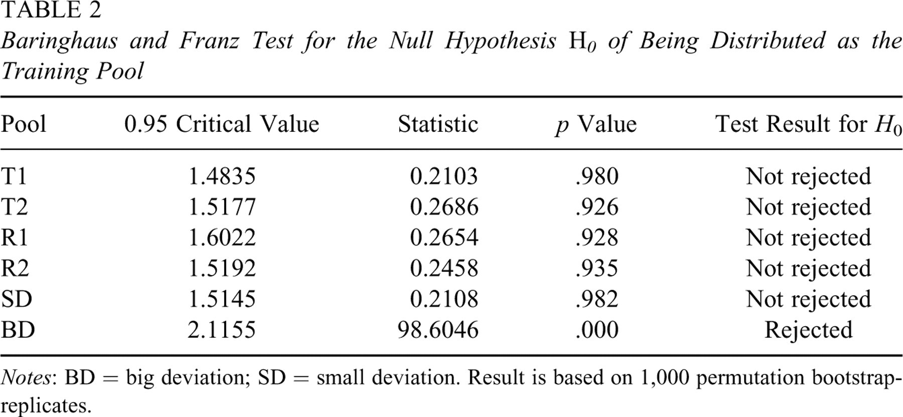
Notes: BD = big deviation; SD = small deviation. Result is based on 1,000 permutation bootstrap-replicates.
Synthetic Item Pools R1 and R2
Using IPs from the training pool as the set of samples, the Taylor and Thompson (1986) procedure was applied with m = 5 and 3 to generate synthetic pools R1 and R2. Each of these pools was parallel to the training pool as shown in Table 2 with high p values.
Synthetic Item Pools SD and BD
The SD (small deviation) pool in Table 1 was synthesized from T1 by perturbing the a (discrimination) and b (difficulty) parameters of 10 random items. The perturbation was in the range of 0.01, and these 10 items had diverse IEPs. This mimics a situation where some of the items have been compromised and must be replaced by items with similar quality. The big deviation (BD) pool was prepared using a uniform sampling for a and a normal sampling for b, respectively. The BD pool was intended to be a nonparallel pool to the training pool.
Simulation Studies
IEPs of the training pool were first obtained using a simulation procedure. Various extensions of the Sympson and Hetter (1985) procedure were considered. Except the conditional Stocking and Lewis procedure, a population of 10,000 simulees drawn from the standard normal distribution N(0, 1) was used to find IEPs of the training pool. For the conditional multinomial procedure, 5,000 simulees with fixed ability were used for each ability level.
Evaluation of Predicted IEPs
For each test pool (i.e., T1, T2, R1, R2, SD, and BD), mean absolute error (MAE) was
calculated to assess the accuracy of MLP predictions. The MAE is defined as follows:
 where ki
is the target IEP simulated from the same SH-type procedure used for the
training pool, and
where ki
is the target IEP simulated from the same SH-type procedure used for the
training pool, and
The performance of ki
and 
 where
where
Experimental Environment
Hardware: A personal computer with Intel Pentium 4/3.0 GHz CPU and 512 MB
memory was used for the simulation studies. Software: The NeuroSolutions software from NeuroDimension Inc. (Gainesville,
FL) was used for MLP implementation, the cramer package under R was adopted
for the Baringhaus and
Franz (2004) multivariate two-sample test, and the rndat
subroutine from IMSL was used for the Taylor and Thompson (1986) random
data generator. MLP environment: The recommended network structure from NeuroSolutions was
experimented and tuned to find a satisfactory structure. Each case was
trained with 100,000 epochs.
Simulation Results
Characteristics of Simulated IEPs
Due to the nature of simulation, IEP fluctuates with the random seed used to start an SH-type procedure. Because the purpose of this study was to find a functional relation k = fP (a, b, c), it was desirable to know how stable the k was, given different random seeds. It turned out that for all variants of the SH procedure except the van der Linden (2003) alternatives, simulated IEPs were quite stable regardless of the seeds used. Take the training pool as an example, 10 runs of the original SH procedure were conducted with different seeds. For each item, the standard deviation of the 10 simulated IEPs was close to 0. The maximum standard deviation from the 360 items of the pool was 0.019323, and the mean of these standard deviations was 0.001163. For the van der Linden (2003) alternatives with γ = 0.15, simulated IEPs depended critically on the seed used to start a simulation. For example, with two different random seeds, the SH procedure produced two sets of IEPs with a maximum absolute difference of 0.0415, whereas the van der Linden procedure produced two such sets with a maximum absolute difference of 0.1777.
The Sympson and Hetter (1985) Procedure
The original SH procedure using item information to select items and Equation 2 to
update IEPs was implemented with r
max = 0.2 and a test length of 20. With simulated IEPs from the training
pool, a MLR was first applied to investigate a linear relationship between IPs and
IEPs as follows:
 where each regression coefficient was significant with
p < .001 and the unadjusted R
2 was .400. This indicates all three IPs are strong predictors for
k. The negative coefficient of a implies that if
an item is more discriminatory, it should be controlled with a tighter IEP to guard
against overexposure. The regression formula was used to predict IEPs from IPs of the
test pools. The predicted IEPs were further trimmed to be in the range of
(r
max, 1). Then, predicted IEPs were evaluated as outlined above with
results summarized in Table
3. It is observed that the MLR formula, though very elucidative, did not
perform well on the test pools. Many items were overexposed and one could hardly tell
any differences between parallel and nonparallel tools except that the nonparallel BD
pool used significantly fewer items than the parallel pools.
where each regression coefficient was significant with
p < .001 and the unadjusted R
2 was .400. This indicates all three IPs are strong predictors for
k. The negative coefficient of a implies that if
an item is more discriminatory, it should be controlled with a tighter IEP to guard
against overexposure. The regression formula was used to predict IEPs from IPs of the
test pools. The predicted IEPs were further trimmed to be in the range of
(r
max, 1). Then, predicted IEPs were evaluated as outlined above with
results summarized in Table
3. It is observed that the MLR formula, though very elucidative, did not
perform well on the test pools. Many items were overexposed and one could hardly tell
any differences between parallel and nonparallel tools except that the nonparallel BD
pool used significantly fewer items than the parallel pools.
Evaluation of MLR With the SH Procedure
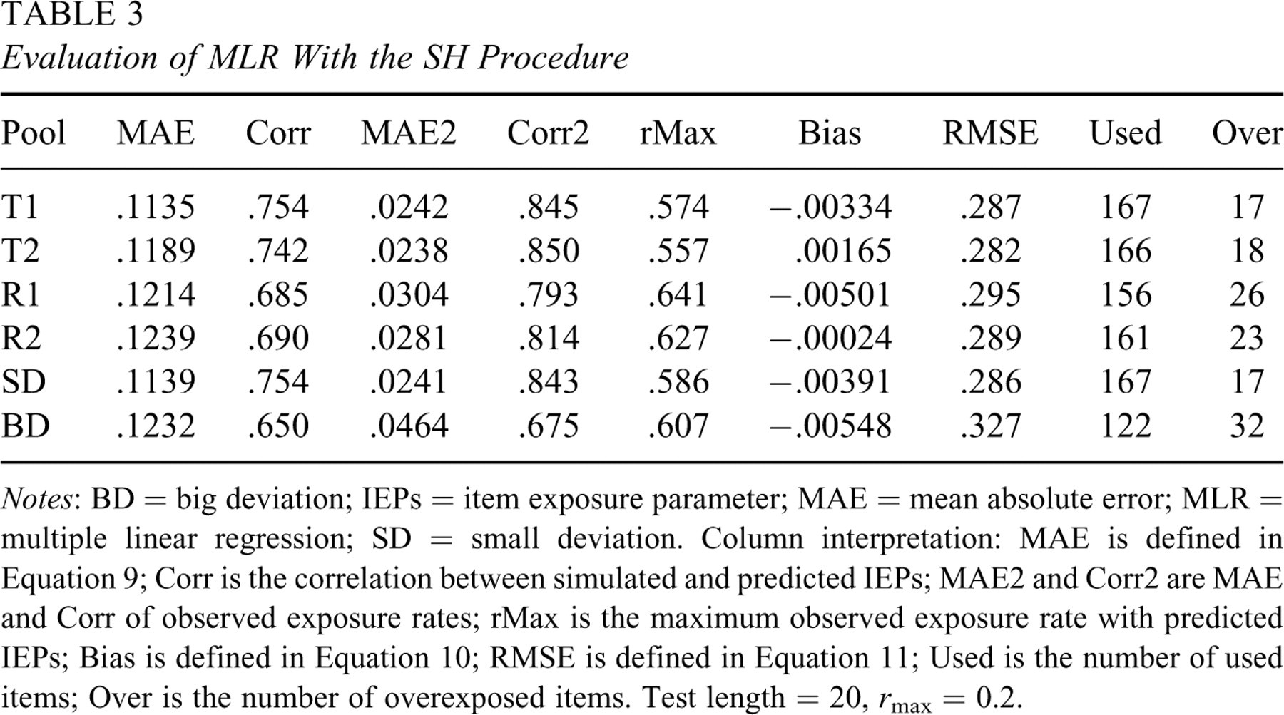
Notes: BD = big deviation; IEPs = item exposure parameter; MAE = mean absolute error; MLR = multiple linear regression; SD = small deviation. Column interpretation: MAE is defined in Equation 9; Corr is the correlation between simulated and predicted IEPs; MAE2 and Corr2 are MAE and Corr of observed exposure rates; r max is the maximum observed exposure rate with predicted IEPs; Bias is defined in Equation 10; RMSE is defined in Equation 11; Used is the number of used items; Over is the number of overexposed items. Test length = 20, r max = 0.2.
The naive linear regression in Equation 12 may not be able to track
a nonlinear relationship between IPs and IEPs well. Because IEP is in a sense a
proportion, a log odds transformation was performed on IEP with the result regressed
by a MLR, that is, log(k/(1 − k)) = β0 +
β1
a + β2
b +β3
c. Notice that this log odds transformation has resulted in a one
layer neural network as
Based on the idea that tightly controlled items should receive larger weights in
training, another weighted MLR was considered. Each item in the training pool
received a weight depending on its IEP as follows:
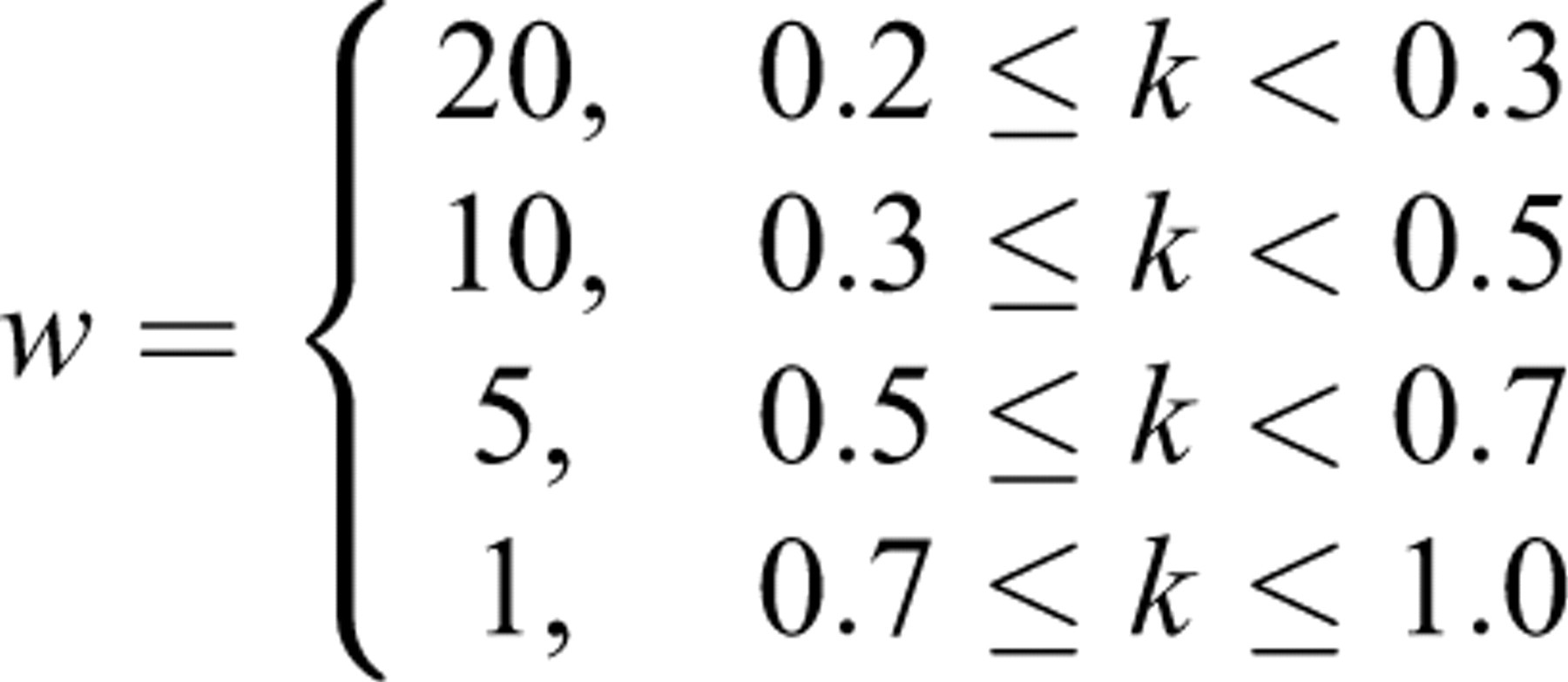 This weight assignment was determined subjectively. Using the weighted
MLR from the training pool, IEPs of T1 were again predicted and assessed as before.
The MAE between simulated and predicted IEPs increased from .1135 (in MLR) to .1463
(in weighted MLR), and the correlation stayed about the same (.754 for MLR vs. .751
for weighted MLR). A particular difficulty in weighted MLR was to set proper weights
for training examples. The same weight assignment for logistic regression improved
the results only slightly from the unweighted logistic regression.
This weight assignment was determined subjectively. Using the weighted
MLR from the training pool, IEPs of T1 were again predicted and assessed as before.
The MAE between simulated and predicted IEPs increased from .1135 (in MLR) to .1463
(in weighted MLR), and the correlation stayed about the same (.754 for MLR vs. .751
for weighted MLR). A particular difficulty in weighted MLR was to set proper weights
for training examples. The same weight assignment for logistic regression improved
the results only slightly from the unweighted logistic regression.
Because of the unsatisfactory results of MLR and logistic regression, MLP was used to find a functional relation between IPs and IEPs. Based on the trained MLP, IEPs of the test pools were predicted and evaluated as before with results summarized in Table 4. This MLP relation performed quite differently on parallel and nonparallel pools. The MAE between simulated and predicted IEPs of parallel pools was several orders smaller than that of the BD pool. Moreover, the correlation value was much higher and close to 1.0 on parallel pools. The same conclusion can be said for MAE and correlation of the observed exposure rates (the MAE2 and Corr2 columns). The five parallel pools had a maximum observed exposure rate less than .27 using around 170 items, whereas the BD pool had a maximum observed exposure rate of .723 using 114 items. Bias, RMSE, and item usage were about the same size on parallel pools when simulated or predicted IEPs were used in an operational CAT. Thus, the functional relation discovered by MLP preserved key characteristics of CAT operations on parallel pools.
Evaluation of MLP With the SH Procedure
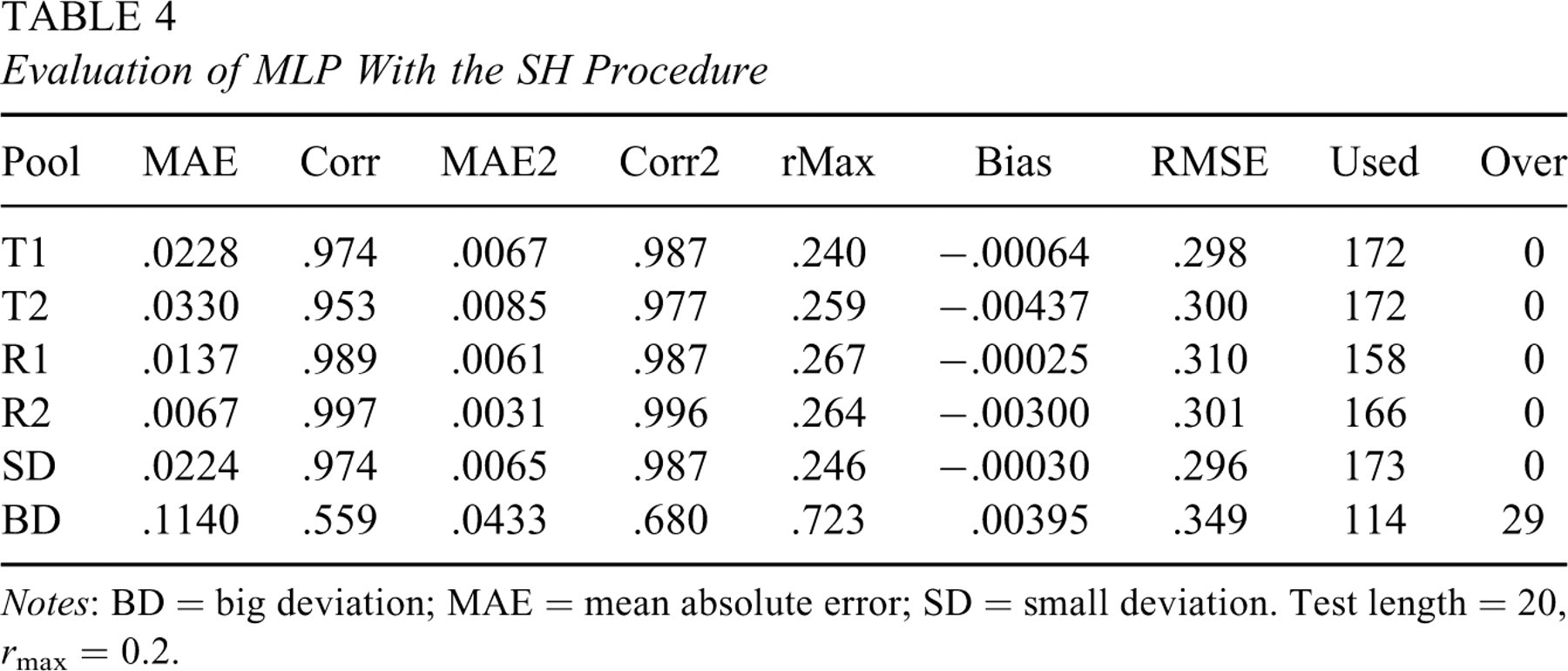
Notes: BD = big deviation; MAE = mean absolute error; SD = small deviation. Test length = 20, r max = 0.2
To further examine the knowledge-based approach, similar experiments with the SH procedure were conducted with a tighter exposure control (r max = 0.1) or a longer test length (l = 30). Results for the tighter control are listed in Table 5, and results for the longer test length are listed in Table 6. These two experiments used more items to satisfy stricter conditions, but the comparison between simulated and predicted IEPs is similar to that for the basic case. Although MLP has provided good results to estimate IEPs without simulation, unlike MLR in Equation 12, it is difficult to see directly from the MLP relation the effect of a, b, or c on k.
Evaluation of MLP With the SH Procedure
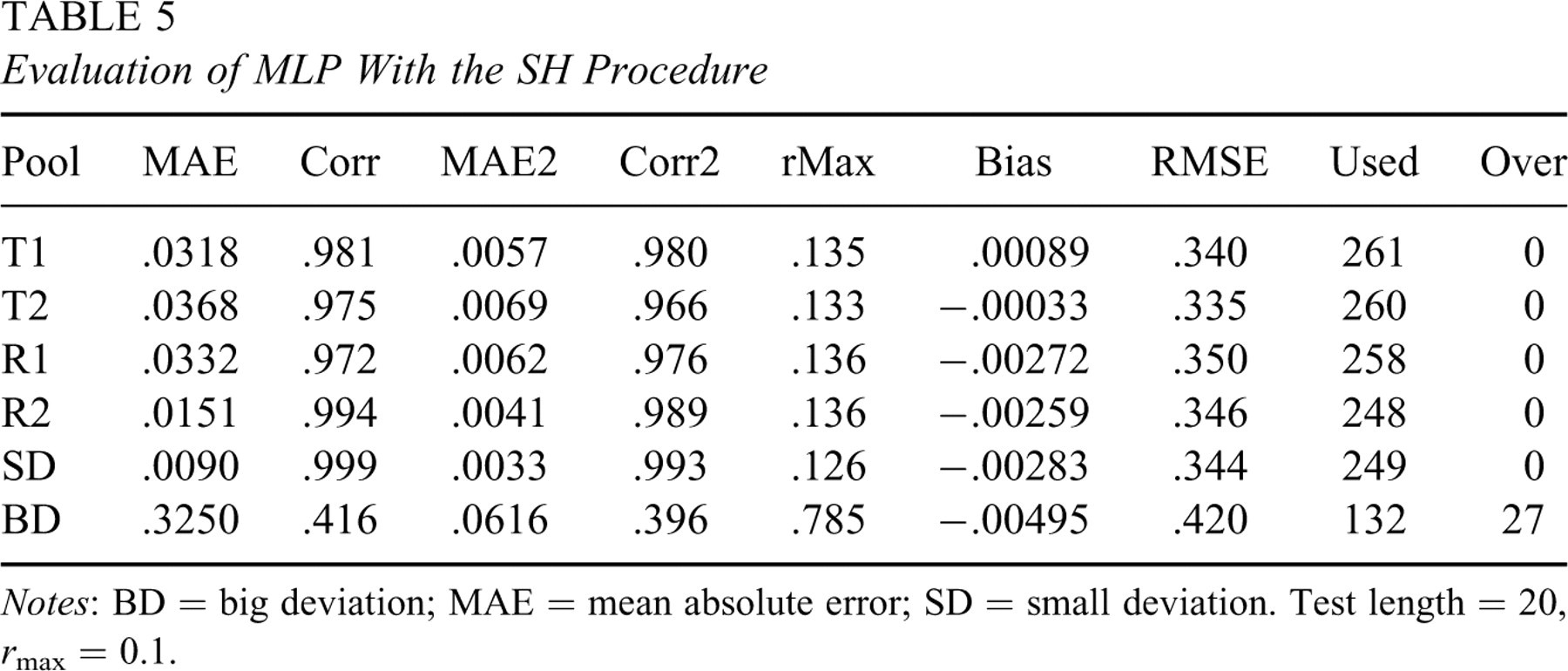
Notes: BD = big deviation; MAE = mean absolute error; SD = small deviation. Test length = 20, r max = 0.1.
Evaluation of MLP With the SH Procedure
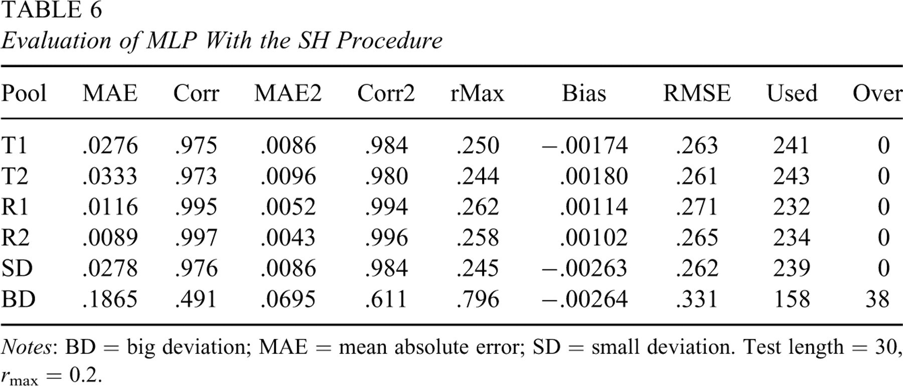
Notes: BD = big deviation; MAE = mean absolute error; SD = small deviation. Test length = 30, r max = 0.2.
The van der Linden (2003) Alternatives
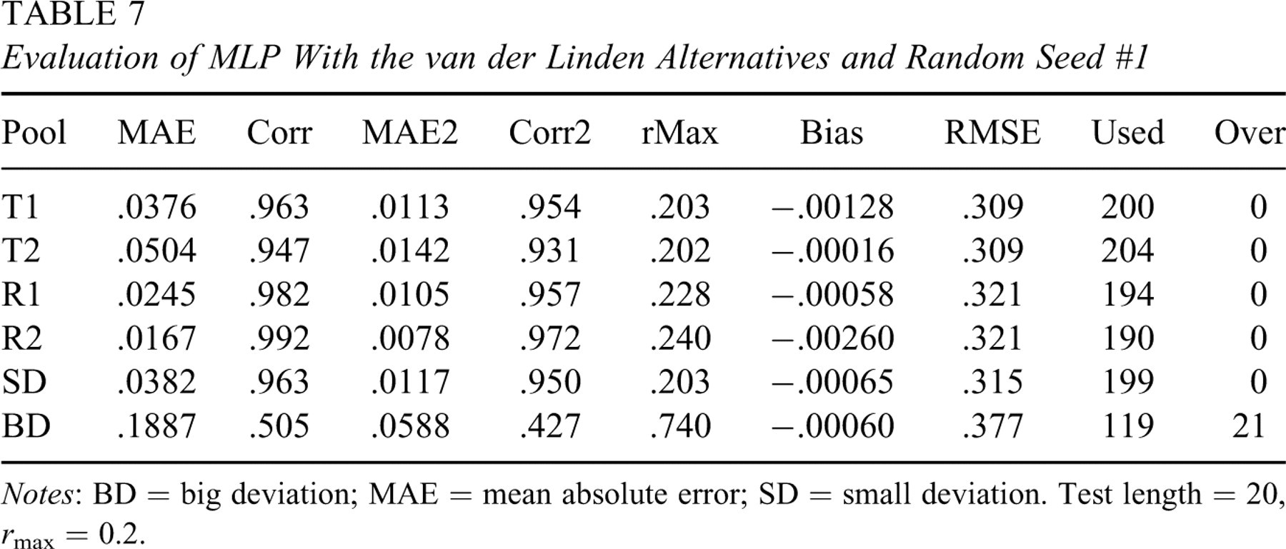
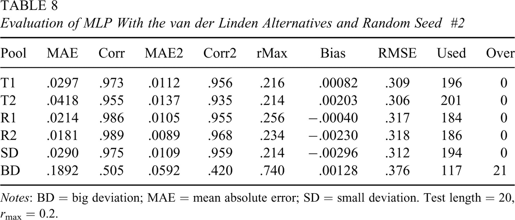
The van der Linden procedure uses item information to select items as the original SH procedure, however, it changes the IEP updating step to Equation 3. Two runs of the van der Linden procedure for the training pool with r max = 0.2, test length = 20 and γ = 0.15 in Equation 3 were conducted. These two runs differed in the random seed used to start the simulation. In the evaluation process, the same seed in a run was used to obtain simulated IEPs of test pools. Predicted IEPs were not trimmed to be greater than r max because simulated IEPs from the van der Linden procedure can be smaller than r max. Results of the MLP approach with the two random seeds are reported in Tables 7 and 8, respectively. In addition, functional relations approximated by MLP performed well on parallel pools and poorly on the BD pool. Maximum observed exposure rate was better controlled and more items were used than the knowledge-based approach for the SH procedure.
Evaluation of MLP With the van der Linden Alternatives and Random Seed #1
Notes: BD = big deviation; MAE = mean absolute error; SD = small deviation. Test length = 20, r max = 0.2.
Evaluation of MLP With the van der Linden Alternatives and Random Seed #2
Notes: BD = big deviation; MAE = mean absolute error; SD = small deviation. Test length = 20, r max = 0.2.
The Unconditional Stocking and Lewis (1998, 2000) Multinomial Procedure
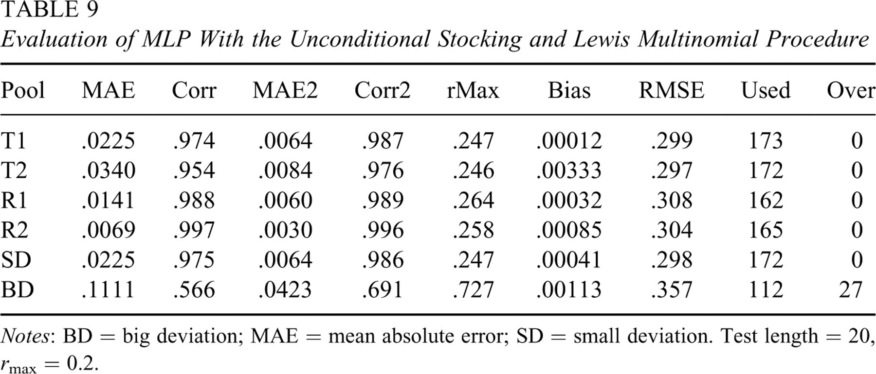
Unlike the van der Linden procedure, the Stocking and Lewis (unconditional or conditional) multinomial procedure modifies the item selection step in the SH procedure while keeping the same IEP updating step in Equation 2. This procedure does not use the maximal item information criterion but rather a normalized multinomial distribution based on a list of candidate items to select items. For the unconditional Stocking and Lewis multinomial procedure, the target exposure rate was set at r max = 0.2 and the test length was 20. Therefore, each list of candidate items had 18 (=360/20) items. Evaluation of the knowledge-based approach is reported in Table 9. The result shows a very similar performance as the SH procedure in every respect.
Evaluation of MLP With the Unconditional Stocking and Lewis Multinomial Procedure
Notes: BD = big deviation; MAE = mean absolute error; SD = small deviation. Test length = 20, r max = 0.2.
The Conditional Stocking and Lewis (1998, 2000) Multinomial Procedure
For the conditional Stocking and Lewis multinomial procedure, the ability scale was discretized into 15 levels: θ m = −3.5 +(m − 1) × 0.5, m = 1, …, 15.. A target exposure rate was set at r max = 0.2. The test length was 20, and each list of candidate items had 18 items. Because of the tremendous amount of CAT simulations (5,000 × 15 = 75,000 for an iteration), this procedure was the most expensive one to find simulated IEPs.
To accommodate the ability factor in MLP, inputs were expanded to include a θ variable. Thus, a functional relation k = fP (a, b, c, θ) was sought using a training set of 360 × 15 = 5,400 examples from the training pool. The θ variable was replaced by the formula −3.5 + (m − 1)× 0.5 during the training and operational phases of MLP. Results in Table 10 show that the performance of this knowledge-based approach was excellent. For each parallel pool, the maximum observed exposure rate was 0.21, and substantially more items were used. The nonparallel pool still performed poorly with the predicted IEPs. To examine the precision performance at each ability level, operational CATs were conducted to simulees of ability fixed at −3, −2, −1, 0, 1, 2, and 3. The Bias and RMSE are plotted against the ability level in Figures 2 and 3, respectively. It is observed that, at each ability level, the Bias and RMSE values for the parallel pools were almost the same as those for the training pool. This shows that the predicted IEPs did not degrade the precision of ability estimation at any ability level.
Evaluation of MLP With the Conditional Stocking and Lewis Multinomial Procedure
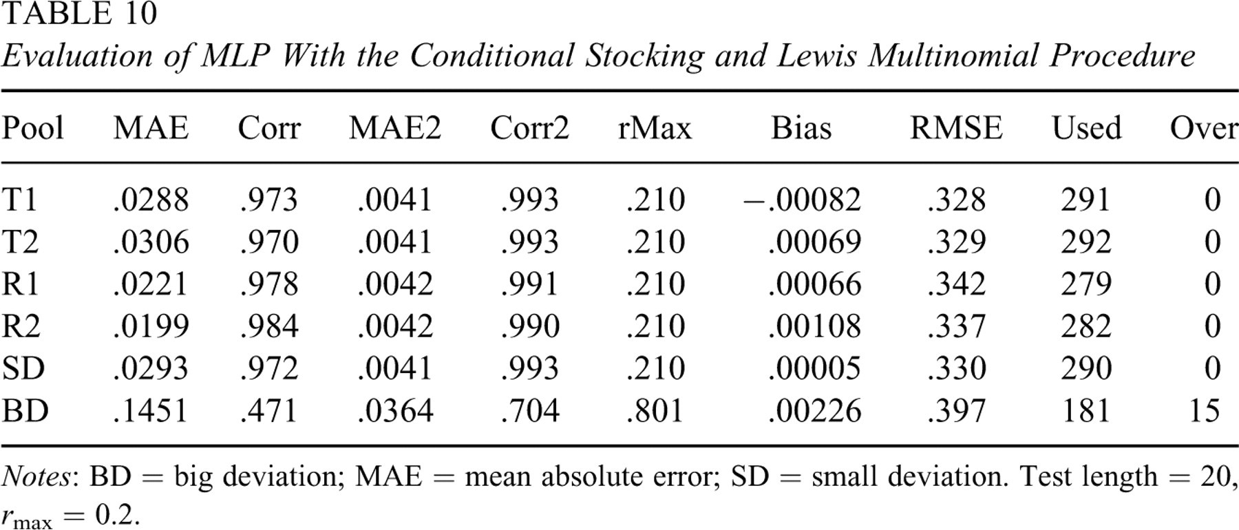
Notes: BD = big deviation; MAE = mean absolute error; SD = small deviation. Test length = 20, r max = 0.2.
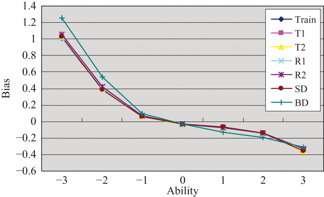
Bias from operational computerized adaptive testings (CATs) conditional on ability level. Training pool uses simulated item exposure parameters (IEPs) from the conditional Stocking and Lewis multinomial procedure; other pools use predicted IEPs.
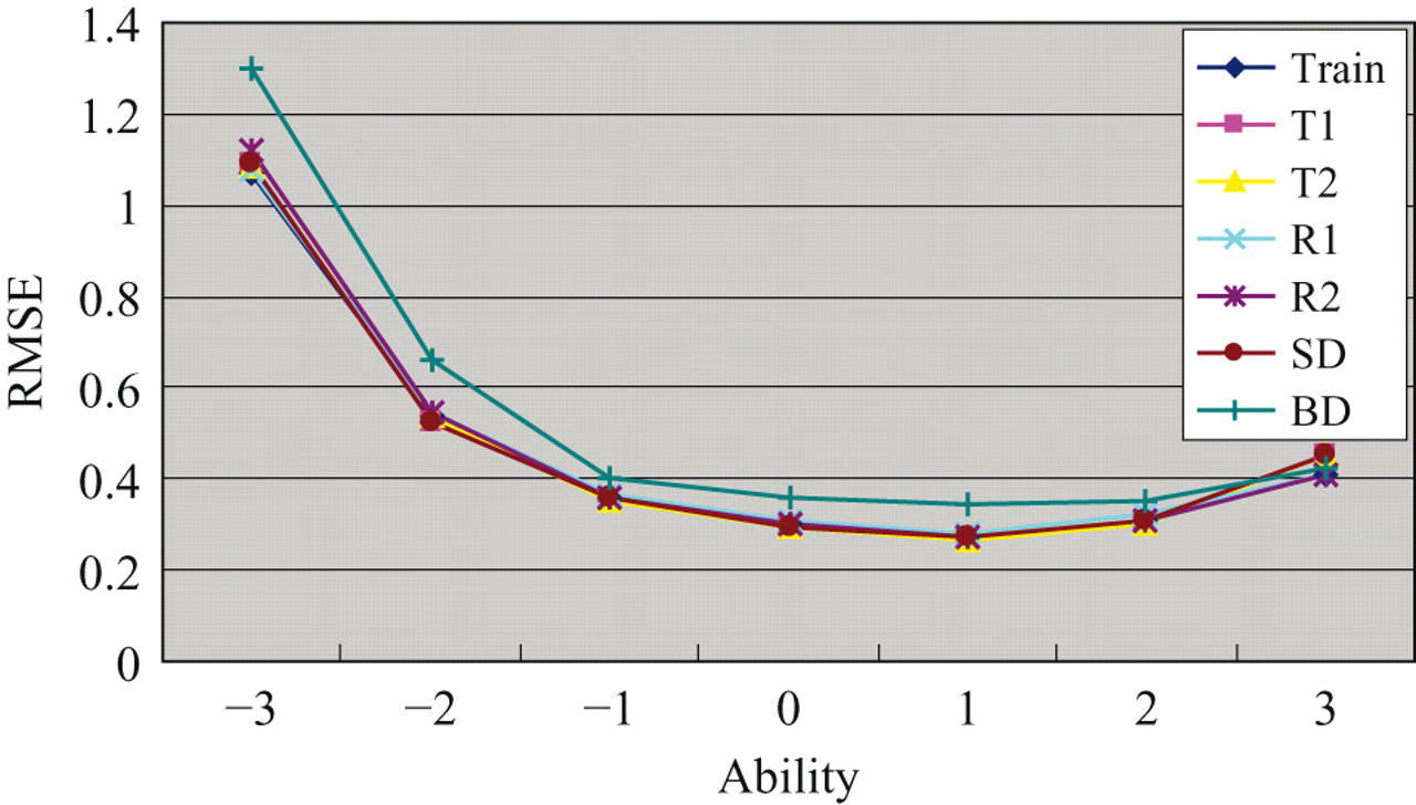
Root mean squared error (RMSE) from operational computerized adaptive testings (CATs) conditional on ability level. Training pool uses simulated item exposure parameters (IEPs) from the conditional Stocking and Lewis multinomial procedure; other pools use predicted IEPs.
The Chen and Lei (2005) Item Exposure and Test Overlap Control
The Chen and Lei procedure modifies the SH procedure using a different IEP updating step in Equation 6 and preserves the item selection step using item information. Using the Chen and Lei (2005) procedure with a target exposure rate of r max = 0.2, a target test overlap rate of T 0 = 0.15 and a test length of 20, IEPs were simulated for the training pool. An MLP was trained with these simulated IEPs and used to predict IEPs of test pools. Evaluation of predicted IEPs is summarized in Table 11. Item exposure and test overlap were controlled pretty well for parallel pools, and this procedure used a few more items than the SH procedure.
Evaluation of MLP With the Chen and Lei Procedure
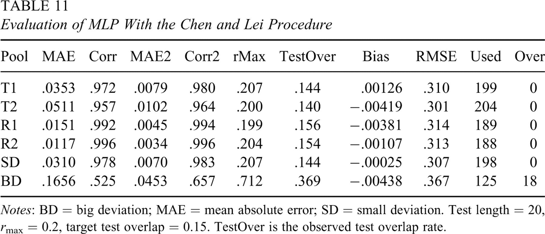
Notes: BD = big deviation; MAE = mean absolute error; SD = small deviation. Test length = 20, r max = 0.2, target test overlap = 0.15. TestOver is the observed test overlap rate.
A Structural Requirement for Tests—the Content-Balancing Requirement
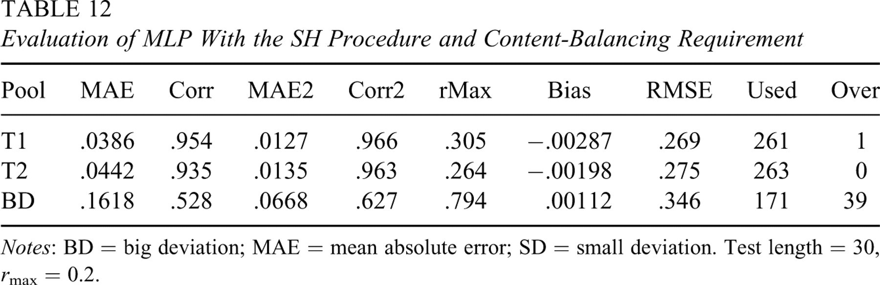
The real pools (training, T1, and T2) contained a content indicator to impose a content-balancing requirement. Six content areas existed in each pool, and the number of items in these areas was 84, 60, 54, 54, 84, and 24 with 7, 5, 4, 5, 7, and 2 items, respectively, to be administered. It was found that subpools of these three pools in each content area were all parallel with high p values (>.8) in the Baringhaus and Franz test. The SH procedure was modified in the item selection step to handle a content-balancing requirement, whereas the original IEP updating step was preserved. To minimize the learning complexity for an ANN, a sequential content selection procedure was implemented, that is, content area s must serve prespecified items before a test moved to the next content area s + 1. In each content area, a computerized adaptive test used the criterion of maximal item information to select items. A target exposure rate was set at r max = 0.2. Inputs to the knowledge-based approach were expanded to include a nominal content indicator s (=1, 2, 3, 4, 5, or 6). Evaluation of predicted IEPs is summarized in Table 12, which shows that the functional relation k = ftraining (a, b, c, s) carried knowledge nicely (badly) from the training pool to parallel (nonparallel) pools. Although the predicted IEPs seemed to perform better in T2 in terms of observed exposure rates, the MAE and Corr actually indicated that MLP had made more precise predictions in T1. A further look into the parallelism of each subpool of content area revealed that T2 had a lower p value (around 0.8) in one area.
Evaluation of MLP With the SH Procedure and Content-Balancing Requirement
Notes: BD = big deviation; MAE = mean absolute error; SD = small deviation. Test length = 30, r max = 0.2.
One may speculate that if each content area is learned separately, a better result may be obtained. That is, a functional relation ks = ks (a, b, c) is learned from the training pool for each content area s and used to predict IEPs of T1 or T2 in that area. Unfortunately, experiments revealed that this approach had worse results than the original approach. This may be explained as follows. Owing to the sequential content selection method, the functional relation ks depends on its precedent relations, that is, ks = ks (a, b, c, ks − 1, …, k 1), because item selections in the s th area depend on the ability estimation up to the (s − 1)th area and IEPs in an area restrain how items are selected in that area and thus can influence ability estimation. Therefore, the s th functional relation ks depends on IPs not only from the s th content area but also from previous areas.
The Chang and Ying (1999) Stratification Procedure
The Chang and Ying (1999) procedure is very similar to the sequential content selection procedure described above, only this time a content area is called a stratum. Leung, Chang, and Hau (2002) implemented an a-stratified design with a modified SH procedure to control item exposure. Their procedure deviated from the Sympson and Hetter (1985) procedure in two places: (a) the difficulty parameter b was used to select items; and (b) a multiplicative form k′ = ck was used to update IEPs. The factor c was set to 1.04 (0.95) when the observed exposure rate of an item was smaller (greater) than the target r max. In the following, two experiments were conducted to implement the a-stratification procedure. Both experiments used the same stratification for item pools, but they differed in the item selection step in strata. The first experiment followed the original SH procedure to control item exposure in a stratum, and the second experiment adopted the mechanism in Leung, Chang, and Hau.
The training pool was partitioned into four strata according to the discrimination parameter a. Each stratum had 90 items and supplied 5 items to a test-taker. During the first stage of a test, items were selected and administered using the original SH procedure on the first stratum of 90 items. After five items had been administered from this stratum, the same procedure moved to the next stratum until 20 items were administered to a test-taker. The target exposure rate was set at r max = 0.2. For the MLP approach, input variables consisted of four variables a, b, c, and s. The nominal variable s (=1, 2, 3, or 4) was used to indicate the stratum number. Evaluation of the predicted IEPs is summarized in Table 13. A few items were overexposed for parallel pools and Corr value decreased to 0.841. Because of the a-stratification step, lower degree of subpools parallelism as indicated by low p values in Table 14 had partially contributed to this effect. For example, T2 and SD had low p values in a few strata. Incidentally, they also had higher MAE and lower Corr than the other parallel pools.
Evaluation of MLP With the Chang and Ying a-Stratification Procedure
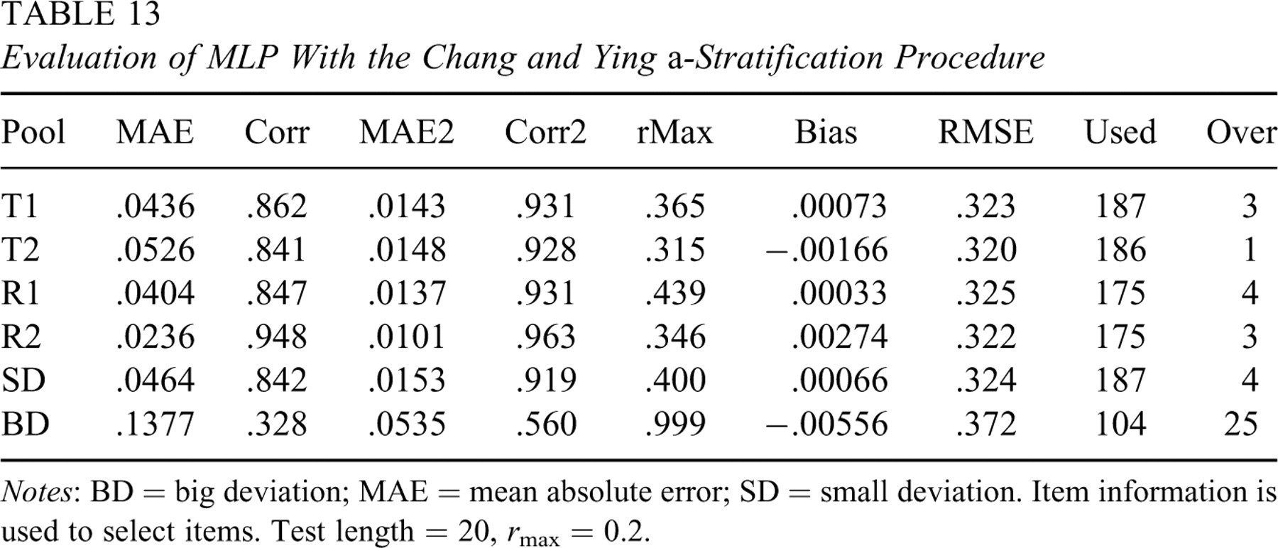
Notes: BD = big deviation; MAE = mean absolute error; SD = small deviation. Item information is used to select items. Test length = 20, r max = 0.2.
Baringhaus and Franz Test for the Degree of Parallelism Between Corresponding Stratum of the Training and Test Pools
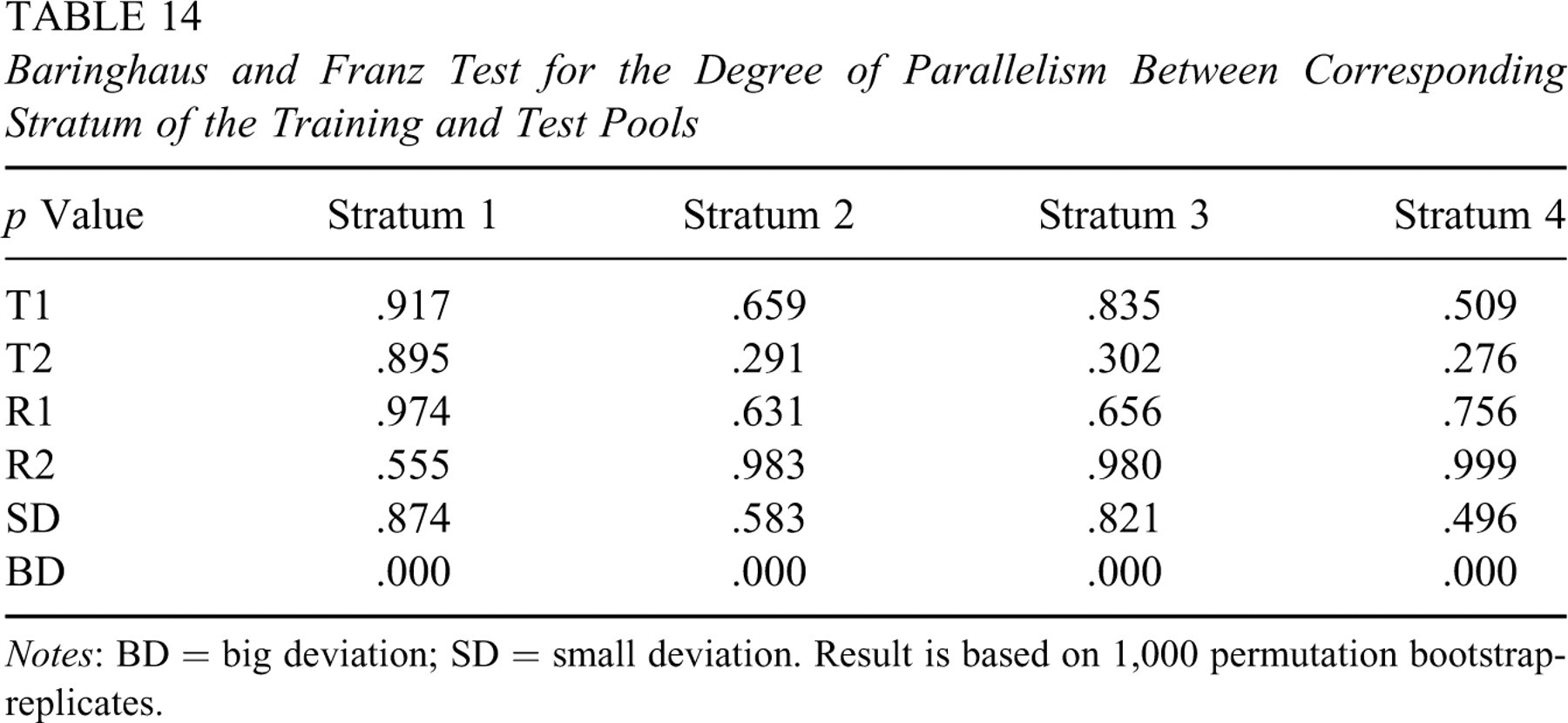
Notes: BD = big deviation; SD = small deviation. Result is based on 1,000 permutation bootstrap-replicates.
The above stratification approach used a few more items than the original SH procedure without stratification. When the difficulty parameter b was used to select items, item utilization improved substantially. In this second experiment, item with the difficulty parameter closest to the estimated ability of a test-taker was selected for administration consideration. It was found that the multiplicative form k′ = ck used to update IEPs in Leung, Chang, and Hau (2002) was inefficient, thus this experiment used Equation 2 to update IEPs. The results are summarized in Table 15, which shows very similar phenomena as the previous experiment with two exceptions: (a) more items were used; and (b) RMSE was higher. Therefore, using the difficulty parameter to select items improved item usage, but it also made ability estimation less efficient.
Evaluation of MLP With the Chang and Ying a-Stratification Procedure
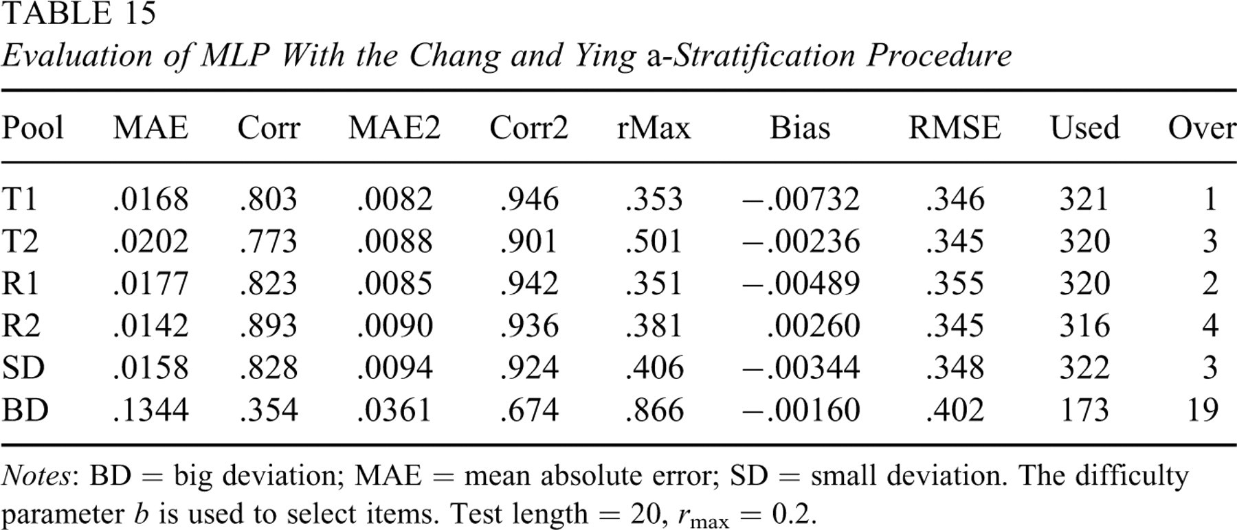
Notes: BD = big deviation; MAE = mean absolute error; SD = small deviation. The difficulty parameter b is used to select items. Test length = 20, r max = 0.2.
Discussions
CAT cannot be implemented effectively unless item exposure is well controlled. The Sympson and Hetter (1985) procedure and its various modifications are commonly used in real applications or CAT studies to control item exposure. The SH-type procedures find stabilized IEPs through iterative simulation. A knowledge-based approach using ANNs has been proposed in this study to approximate a functional relation between IPs and IEPs of a training pool so that IEPs of parallel pools can be directly estimated without tedious simulation.
An operational definition of parallel pools was given using statistical attributes of the multivariate samples formed by IPs of item pools. Three real pools and four synthetic pools, together with the SH procedure and its many extensions, were investigated in this study to verify the proposed knowledge-based approach. It was found that the knowledge-based approach provided good results for item exposure control based on the original Sympson and Hetter (1985) procedure, the van der Linden (2003) alternatives and the unconditional Stocking and Lewis (1998, 2000) multinomial procedure. This knowledge-based approach provided excellent results for the conditional Stocking and Lewis multinomial procedure and the Chen and Lei (2005) procedure to control both item exposure and test overlap.
The knowledge-based approach worked satisfactorily for the SH procedure with a content-balancing requirement and less satisfactorily for the Chang and Ying (1999) a-stratification procedure. For these two types of exposure control, a nominal variable indicating the content area or stratum number was added to the list of independent variables. Several learning difficulties need to be investigated to improve the performance of the knowledge-based approach. For example, a previous reasoning argues that IEPs in the sth stage depend on IEPs of previous stages. Thus, a naive input form (a, b, c, s) may not be able to capture this intricacy efficiently. A further causality study is needed to design more efficient predictors for IEPs in multistage item selection mechanisms. Another difficulty involves the degree of parallelism in each subpool of content area or stratum, and this is especially serious with the a-stratification procedure.
In general, p value in the Baringhaus and Franz test can be used to indicate the degree of parallelism between pools. However, how robust is this indicator in CAT applications remains to be verified in future studies. For examples, using tens of neighbors in the Taylor and Thompson (1986) procedure, item pools with varying degrees of parallelism to the training pool were generated with the p value ranging from .010 to .776. When the knowledge-based approach was applied to the original SH procedure with r max = 0.2 and test length = 20, it was found that, even with the p value as low as .010, the MLP functional relation k = f training (a, b, c) generalized well to these pools (Table 16). However, the impact of lower degree of parallelism seemed to amplify when multistage item selection mechanisms were considered.
Evaluation of MLP With the SH Procedure
Notes: MAE = mean absolute error. Pools are identified by the p value. Test length = 20, r max = 0.2.
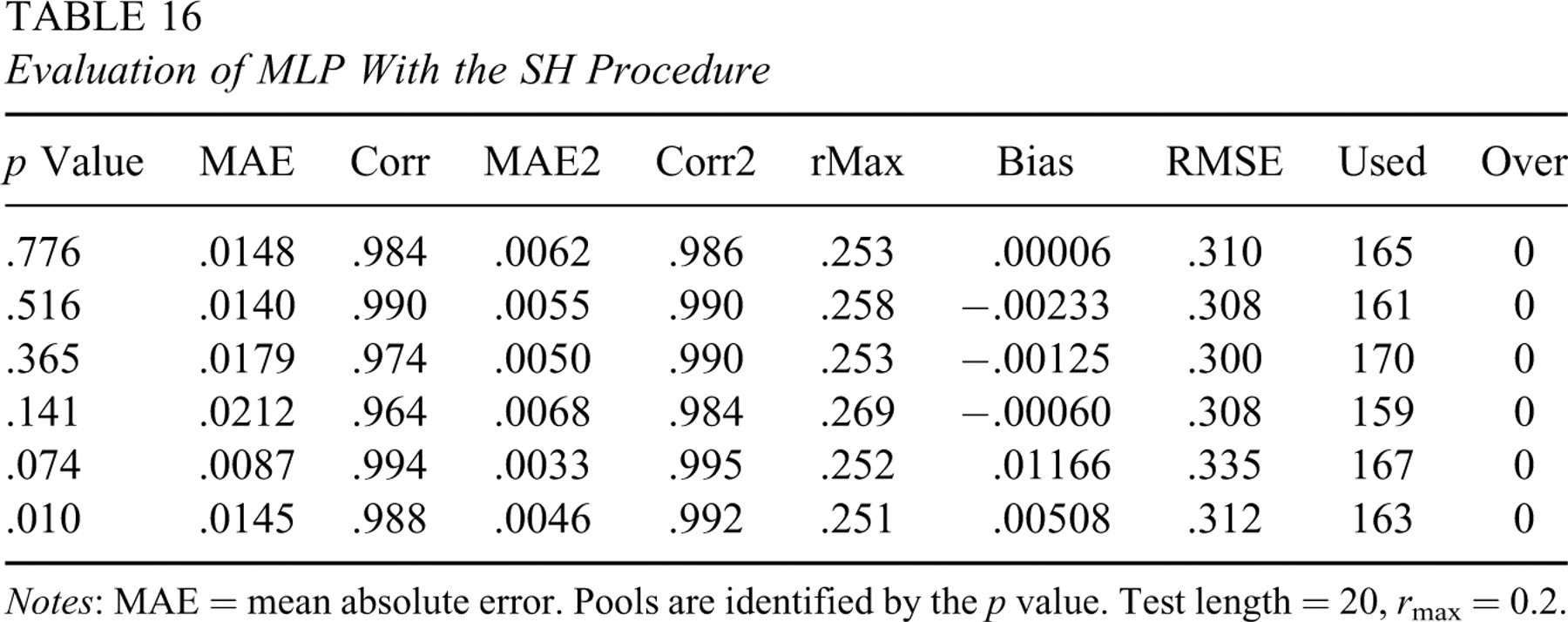
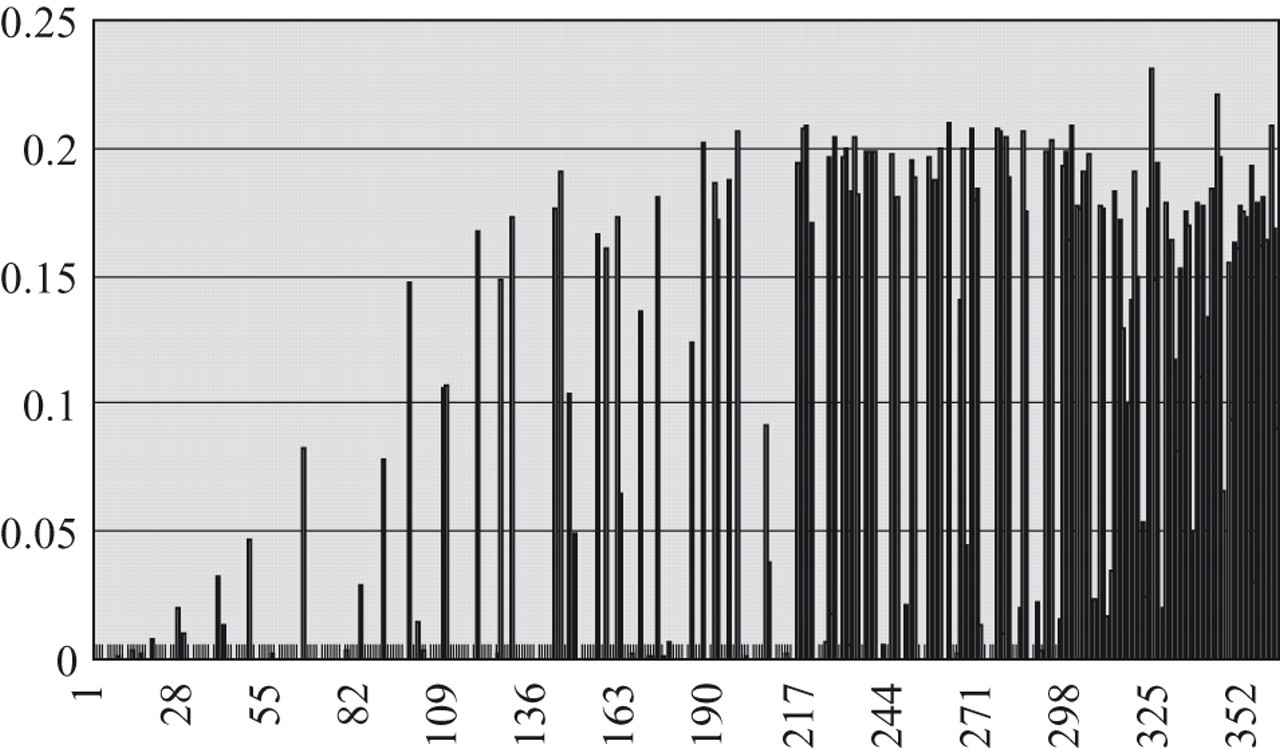
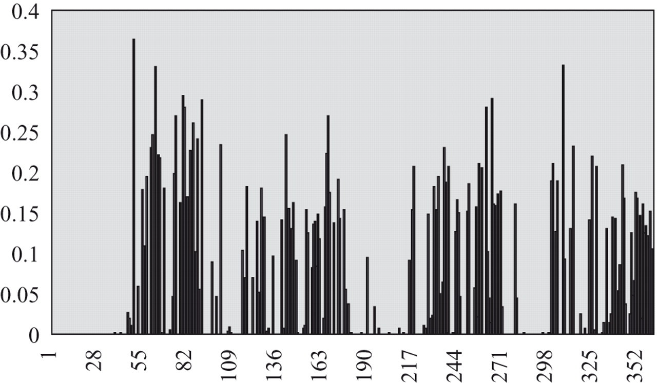
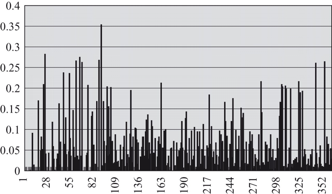
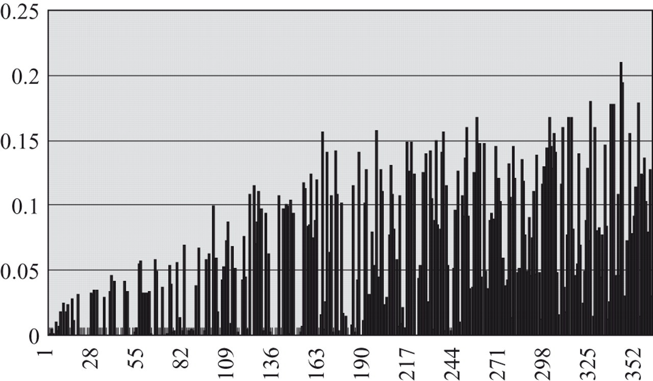
The knowledge-based approach was supposed to faithfully capture the relationship between IPs and simulated IEPs of the training pool. Predicted IEPs and simulated IEPs were expected to have similar item usage on parallel pools, that is, if the simulated IEPs underused many items, so would predicted IEPs. This phenomenon has been observed for all procedures tested in this study. With the SH procedure, Figure 4 shows that predicted IEPs of T1 underused many items with low discrimination parameter. When the a-stratification procedure was implemented with the SH procedure in each stratum, item usage was spread to all strata (Figure 5). However, this procedure still underused many items and tended to use highly discriminatory items in each stratum. Figure 6 shows results for the a-stratification procedure with the difficulty parameter to select items. More items were used across the entire spectrum of the discrimination parameter. However, this procedure also produced higher RMSE for ability estimation and a few overexposed items. The conditional Stocking and Lewis multinomial procedure used items across the entire spectrum of the discrimination parameter without losing precision of ability estimation or item overexposure control (Figure 7).
Exposure rates for the T1 pool; items are sorted according to the discrimination parameter. Predicted item exposure parameters (IEPs) are used with the Sympson and Hetter procedure.
Exposure rates for the T1 pool; items are sorted according to the discrimination parameter. Predicted item exposure parameters (IEPs) are used with the Chang and Ying a-stratification procedure. Item information is used for item selection.
Exposure rates for the T1 pool; items are sorted according to the discrimination parameter. Predicted item exposure parameters (IEPs) are used with the Chang and Ying a-stratification procedure. The difficulty parameter b is used for item selection.
Exposure rates for the T1 pool; items are sorted according to the discrimination parameter. Predicted item exposure parameters (IEPs) are used with the conditional Stocking and Lewis multinomial procedure.
Based on all evaluation criteria, the conditional multinomial procedure is deemed the best application of the knowledge-based approach. Incidentally, the conditional multinomial procedure was also the most expensive procedure to implement, and the knowledge-based approach has provided a practical solution to implement this procedure on parallel pools.
This knowledge-based approach to item exposure control considered mechanisms that needed the SH-type procedure to derive stabilized IEPs. Item exposure controls that did not need any IEPs were not covered in this study. For example, owing to the fact that the discrimination parameter and the difficulty parameter often are positively correlated, Chang, Qian, and Ying (2001) proposed an a-stratified multistage procedure with b blocking. The main idea was to make sure that each stratum had a balanced distribution of b values to guarantee a good match of estimated ability for different test-takers. The a and b parameters of the training pool had a correlation value of .476. Because this a-stratification with b blocking procedure did not need any IEPs to control item exposure, the knowledge-based approach had nothing to learn.
Readers are reminded that the knowledge-based approach in this study was applied to parallel pools defined primarily with statistical attributes. The content-balancing requirement, as a nonstatistical structural requirement, was also considered. As a professional test may include thousands of statistical and nonstatistical constraints on item pools (Ariel et al., 2004), future studies may focus on expanding the knowledge-based approach to cover more requirements on item pools.