
Abstract
In this article, a latent trait model is proposed for the response times in psychological tests. The latent trait model is based on the linear transformation model and subsumes popular models from survival analysis, like the proportional hazards model and the proportional odds model. Core of the model is the assumption that an unspecified monotone transformation of the response times can be related to latent characteristics of the test taker. The model can be interpreted in terms of an information accumulation process, according to which test takers acquire information until they are able to respond. The rate of information accumulation can be related to the transformation function of the response times. In order to avoid strong distributional assumptions, the rate of information acquisition is approximated in a piecewise manner by a positive spline. The model can be calibrated with marginal maximum likelihood estimation. This allows a standard test of model fit as will be shown. The proposed approach to model estimation and model evaluation is investigated in a simulation study. Finally, the utility of the model is demonstrated in three real data sets.
Introduction
In computer-based tests, one usually records not only the responses but also the times needed to give the responses. When analyzing response time data, one usually observes that individuals differ systematically in their response times. This allows for an alternative characterization of the test taker’s performance in terms of his or her work pace, which is, at least to a certain extent, a manifestation of his or her speed of information processing. How response times in psychological tests should be modeled and what can be gained by doing so, however, is an open question.
There is broad consensus that response times in tests should be modeled with a latent trait model similar to the responses, which are analyzed with item response models by default. However, this is the only consensus that exists in this field, and different opinions exist about the best approach to response time modeling in tests. A first disagreement refers to the question of whether one should model responses and response times separately, with two different and unrelated latent trait models, or whether one should model responses and response times jointly, using a common model for both quantities. Not all possible uses of test response times require a joint model, although sometimes jointly modeling responses and response times is more efficient or has greater power when testing hypotheses. Another, somewhat related controversy concerns the structure one considers adequate for the joint distribution of the responses and response times
We do not try to give an answer to the best modeling approach in this article. All mentioned approaches have advantages and disadvantages. The strength of cognitive process models is their interpretability, as components of the model are closely related to elements of the response process (van der Maas, Molenaar, Maris, Kievit, & Borsboom, 2011). This can improve psychological assessment and turn the models into attractive research tools for investigating characteristics of the response process. Furthermore, the close relation to the response process partly justifies the assumptions one makes about the response time distribution. However, one must not forget that these process models were originally supposed for simple decision tasks, mimicking optimal decision devices at lower neuronal levels. Responses in tests are the result of multiple knowledge states and different strategies, and the solution process in complex tasks might not be represented adequately by these models. Besides, there is a contradiction between the wish for a specific model of the response process on one side and the need for a general, widely applicable measurement model on the other side. Conventional latent trait models are statistical models without a very close relationship to the response process and without a profound interpretation in psychological terms. They are more or less atheoretical in nature, not being derived from precise assumptions about the response process. However, such models are flexible, have been used as measurement models successfully for a long time, and are statistically tractable in the typical sample sizes available to test developers. Besides, even though standard latent trait models are inferior to process models with respect to interpretability, they do not necessarily have less predictive power when predicting external criteria (van der Maas et al., 2011). Nevertheless, interpretability and flexibility do not necessarily exclude each other. A model somewhat in between these two poles, more flexible than typical process models and loosely based on assumptions about the response process, might combine the advantages of both approaches.
In this article, we present a flexible response time model, which can be interpreted in psychological terms, as its components are related to elements of the assumed response process. More specifically, the model is derived from the assumption that individuals accumulate information over time and respond as soon as their level of information has reached a critical threshold. As a consequence, the model can be used in order to assess the temporal acquisition of information. The presented model is for the response times only, but it should be seen as a building block in a larger framework. It can be used as a measurement model to derive the latent work pace of an individual from his or her response times. It can be combined with a latent trait model for the responses according to the hierarchical framework of van der Linden (2007), which is based on the factorization
The outline of this article is as follows. First, the response time model will be described. Then, an approach to model calibration will be sketched as well as some tests concerning model fit. The performance of the proposed estimation approach and the tests of model fit will be evaluated in a simulation study. Finally, the model will be applied to three real data sets.
A Response Time Model Based on the Linear Transformation Model
In tests, one is usually interested in assessing the knowledge of an individual. This knowledge, however, is only coarsely assessed when responses are scored as correct or incorrect, as this only allows the classification of the knowledge as sufficient or insufficient to give the correct response. It could be beneficial to model the solution process in more detail, in order to distinguish different solution strategies, detect differential item functioning, or assess measurement invariance, for example. This can be accomplished by the usage of response times as will be shown in the following paragraphs.
The basic idea of the proposed model is the assumption that individuals accumulate information when working on an item of a test. Information is thereby considered to be a positive random variate, monotonously increasing over time. In the following, it is assumed that the level of information I
gi
(tgi
) reached by individual i with respect to the problem posed by Item g up to time tgi
depends on three quantities. First, the level of information I
gi
(tgi
) depends on the baseline rate of information acquisition

Coefficient β
g
is a regression coefficient that regulates the strength the latent trait exerts on the process of information accumulation. Taking the antilog of both sides reveals that exp(β
g
θ
i
) is related multiplicatively to the accumulated information via increasing or decreasing the baseline rate of information acquisition proportionally. Note that Equation 1 contains no intercept parameter, as an intercept parameter can be absorbed into the baseline rate
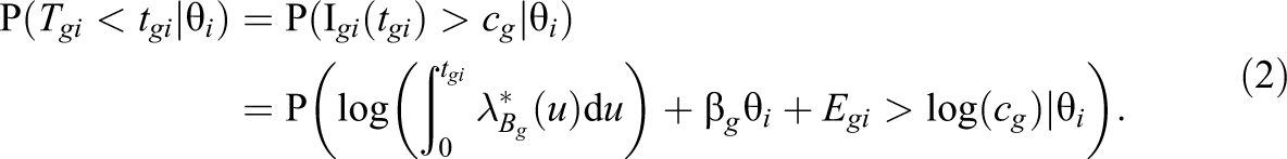
Each item is associated with a critical level of information cg that has to be reached before one is in the position to give a response. This represents the information demand of the item, not under control of the individual. Note that this conception of the solution process is similar to the motivation of the two-parameter logistic model, which can be derived from the assumption that a continuous variable is dichotomized at an item-specific hurdle (Wirth & Edwards, 2007). As a response is given as soon as the information demand cg has been reached, the cumulative distribution function of the response time Tgi in Item g for an individual with work pace θ i follows from Equation 1 as:
Defining

Equation 2 can be rewritten as:
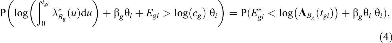
where
Equation 4 implies that the transformation
It is common practice in the linear transformation model to make assumptions about the distribution of the residual term

where τ > 0. Parameter τ determines the exact form of the distribution of the residual. Note that for τ = 1, the distribution simplifies to the density function of the standard logistic distribution. For τ → 0, the distribution converges to the extreme value Type I distribution. Therefore, a model based on Equations 4 and 5 subsumes the proportional hazards model and the logistic odds model as special cases. Although it would be possible to regard τ as item-specific, it appears more reasonable to use the same value for all items of the test. This corresponds to the assumption that the same model class (e.g., proportional hazards model) holds for all items of the test.
The distribution function corresponding to Equation 5 was proposed in a different context by Aranda-Ordaz (1981) as a flexible link function for generalized linear models (see also Royston & Parmar, 2002, for an application of this distribution in survival analysis). It is a nearby choice in case one intends to combine the proportional hazards model and the proportional odds model into a common framework. However, as the distribution of

This follows from a change of variables by the replacement of
The joint distribution of the response times in the g = 1,…, G items of a test follows from the conditional independence assumption. This assumption states that, conditionally on the latent trait, the response times from different items are independent. This is usually justified by the claim that after controlling for the trait θ
i
, which is supposed to be the only systematic influence on the response times, no further systematic relation between the response times remains. In case of conditional independence, the joint distribution of the response times
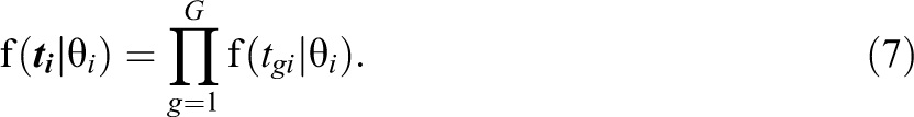
The conditional independence assumption of Equation 7 implies that individuals work with constant work pace throughout the test. This assumption is clearly violated in case individuals start to rush when running out of time at the end of the test. However, in tests with generous time limits, individuals do not have to adapt their way of responding and proceed indeed with the same speed throughout the test according to preliminary findings (van der Linden, Breithaupt, Chuah, & Zhang, 2007; see van der Linden, 2009, for a more thorough discussion of this point).
The proposed model subsumes well-known models of survival analysis, among them the proportional hazards model and the proportional odds model. The proportional hazards model has been proposed as a model for test response times before (see Douglas, Kosorok, & Chewning, 1999; Ranger & Ortner, 2012; C. Wang et al., 2013; C. Wang, Fan, et al., 2013; as well as Loeys, Legrand, Schettino, & Pourtois, 2014). Other applications of the linear transformation model can be found in C. Wang et al. (2013) and Ranger and Kuhn (2013). Ranger and Kuhn (2012) proposed a flexible model for discrete response times in tests that subsumes the proportional hazards model and the proportional odds model. In comparison to these earlier approaches, the current model has some interesting features. First, the proposed model is more flexible than its rivals, as the usage of a flexible distribution allows the integration of several models into one general framework. Second, contrary to the model of Ranger and Kuhn (2012), which is equally flexible, the response times need not to be categorized, such that there is no loss of information and hypothesis about the rate of information acquisition can be tested. Third, the transformation of the response times is not regarded as a nuisance parameter but is explicitly modeled. And fourth, the model can be interpreted in terms of an information accumulation process.
Approximation of the Baseline Rate of Information Acquisition
One of the key quantities of the model is the baseline rate at which an average individual acquires information. This quantity gives more insight into the way individuals process information than simple statistics like the mean or the standard deviation of the response times as noted by Wenger and Gibson (2004); see Aalen and Gjessing (2001) and Burbeck and Luce (1982) for examples of how the rate of information accumulation can be used in order to gain insights into the solution process. When implementing the model, the baseline rate of information accumulation should be modeled without making too strong assumptions about its form. The standard solution for this problem consists in approximating
Several approximations based on positive interpolation or restricted spline functions have been used in the context of response time modeling so far. A first approach consists in modeling the log baseline hazard function (or in our case, the baseline rate of information accumulation) via an ordinary polynomial spline function. Examples for this approach can be found in Kooperberg, Stone, and Truong (1995), Boracchi, Biganzoli, and Marubini (2003), and in the survBayes package of the statistical software environment R (Henschel, Heiß, & Mansmann, 2009). Note that with this approach, one already has to rely on approximations in case of standard distributions like the Weibull distribution, for which reason, sometimes the quantity
In the following, the approach based on the so called I-splines is described in more detail. I-splines are easy to implement, a great advantage in latent trait models that require computer intensive fitting routines. The easiness of their implementation clearly outweighs the fact that I-splines are only a subclass of all piecewise positive polynomials. For most shapes of the baseline rate of information accumulation the I-spline should be sufficient, especially as its flexibility can be increased at will by increasing the number of divisions of the time axis. I-splines are closely related to piecewise polynomial functions as will be explicated in the following. A piecewise polynomial function is a function that is composed of different polynomials. Therefore, the time axis is divided into disjoint segments at prespecified knots κ1, κ2,…, κ K that define the segment borders. In each segment, the piecewise polynomial is represented by distinct polynomials, which are joined together where the segments adjoin. The segment-specific polynomials have to comply with restrictions that guarantee the continuity of the resulting function and of some of its derivatives. Piecewise polynomials can be generated by basis functions. One possible basis is the M-spline basis (Ramsay, 1988). The M-spline basis is defined recursively. Therefore, the domain over which the piecewise polynomial should be evaluated is bordered by two additional boundary knots κ0 and κ K +1. Choices for κ0 and κ K +1 could be the minimal and maximal response time, for example. Each of the additional boundary knots is replicated m times. The number of replications determines the degree of the piecewise polynomial function. Replicating each boundary knot m times yields a piecewise polynomial of degree m − 1 with m − 2 continuous derivatives. Replicating each boundary knot 3 times, for example, yields a function that is continuous, can be represented by a quadratic polynomial in each segment, and has a continuous first derivative. With the augmented knot sequence, the M-spline basis functions can be generated recursively as follows. Define as the start of the recursion the functions:
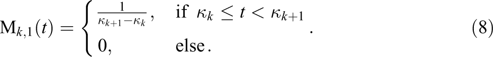
The basis functions of the M-spline basis result by using the recursion:

which has to be used until j = m. This yields m + K basis functions. Applying the recursion, for example, to the augmented knot sequence 0.2, 0.2, 0.2, 0.4, 0.6, 0.8, 1.0, 1.0, and 1.0 gives the M-spline basis functions that are plotted in Figure 1. The M-spline basis functions are nonzero on at most m segments, where they are polynomial functions of degree m − 1. Each M-spline basis function integrates to one.
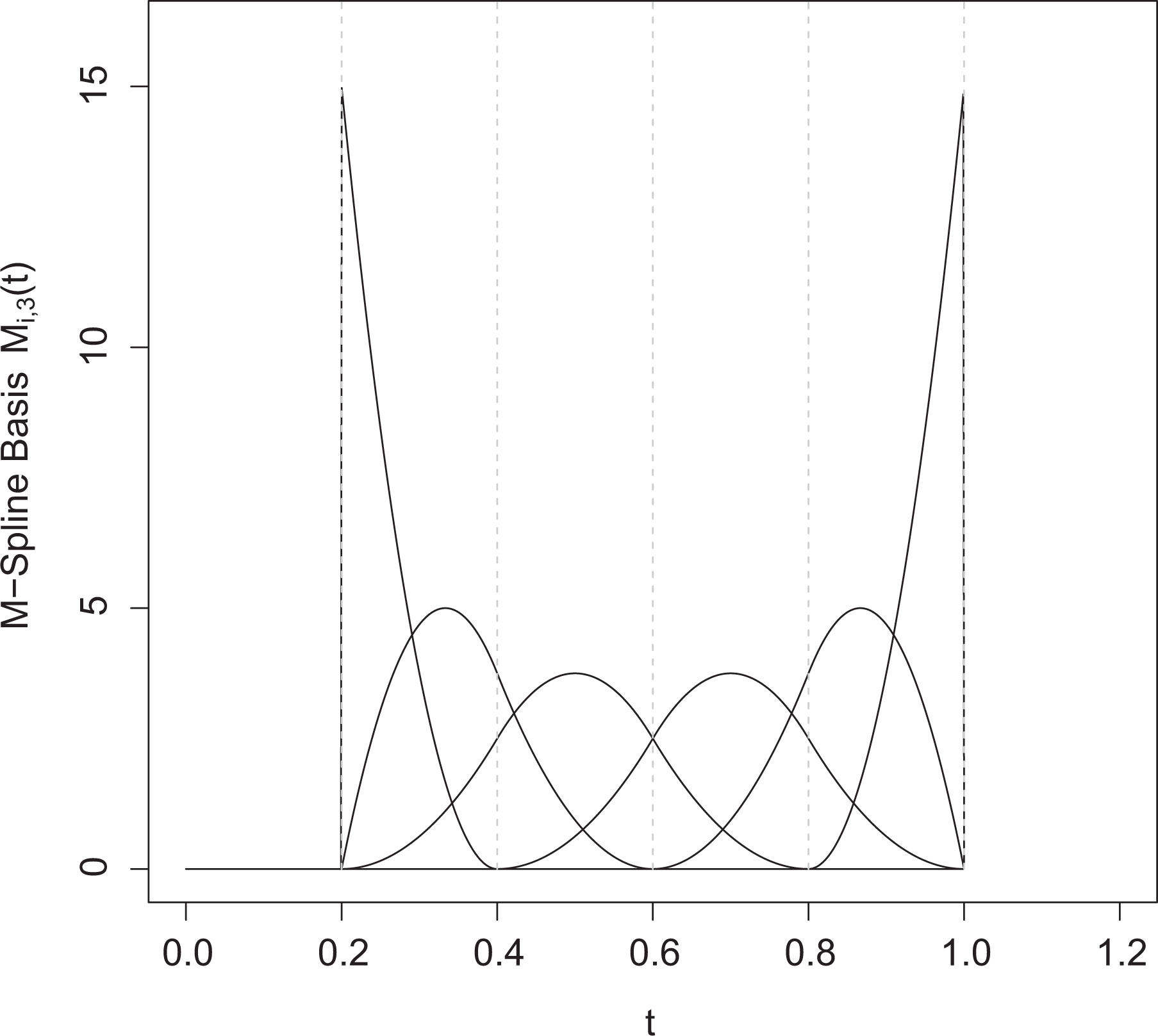
M-spline basis functions corresponding to the knot sequence of 0.2, 0.4 0.6, 0.8, and 1.0, where the boundary knots were repeated 3 times. Each basis function consists of quadratic polynomials with nonzero values over at most three segments.
A piecewise polynomial can be represented by a linear combination of the M-spline basis functions. Summing, for example, the M-basis functions in Figure 1 generates a piecewise quadratic function defined on [0.2; 1.0]. As all M-spline basis functions are positive, the positivity of the resulting piecewise polynomial function follows from the positivity of the weights. This suggests the approximation of the baseline rate of information acquisition by:

where the sum runs over the different M-spline basis functions and

where the integrated M-spline basis functions are usually denoted by I-spline basis functions. Due to the positivity of the M-spline basis functions, the I-spline basis functions and hence their linear combination are monotonously increasing. M-splines have been criticized as being too restricted because they do not cover the whole space of positive piecewise polynomials. For the sake of comparison, we additionally considered an approximation of the baseline rate of information acquisition with a quadratic spline whose positivity was ensured with a technique described by Schmidt and Heß (1987). We also reconstructed the cumulative baseline rate of information acquisition
The number and spacing of the knots has to be determined before the proposed model can be calibrated. Choosing the number of knots comprises a bias-variance trade-off, as more segments promise a better approximation of the baseline rate (less bias) at the cost of higher imprecision of parameter estimates (more variance). With respect to the number of knots, Cai et al. (2011) recommend the usage of 10 to 30 knots, while the publications cited in Liu and Huang (2008) support the view that 8 to 10 knots are usually sufficient. This is also what we recommend. To be on the safe side, one can run a sensitivity analysis and check whether the findings are robust with respect to the number and placement of the knots. Note that alternatively one can successively increase the number of knots until a criterion is optimized (see, e.g., Kooperberg & Stone, 1992, for such an approach). One can also use a large number of basis functions and impose some form of penalty in order to impede overfitting. The usual way of placing the knots is either at equally spaced quantiles or at equally spaced knots between the minimal and the maximal response time (Harrell, 2002).
Model Calibration
Once the number and locations of the knots have been fixed and the M-spline and I-spline basis functions have been determined, the item parameters of the model can be estimated. Instead of calibrating the model with the observed response times, we recommend to censor them at a deliberately chosen lower and upper limit. There are two motivations for censoring. The baseline rate of information acquisition can usually not be recovered very well in the tails of the response time distribution, where observations are sparse. Therefore, it might be wise to prune the response time distribution at some quantiles and estimate the exact form of
The standard approach to model calibration in latent trait models is marginal maximum likelihood estimation. As marginal maximum likelihood estimation is standard practice, it will only be sketched here. Marginal maximum likelihood estimation is based on the marginal response time distribution that can be determined as follows. Let f(θ) be the distribution of the latent trait in the population the test takers are sampled from. Usually, this distribution is the standard normal distribution. Equation 7 specifies the conditional density of the response times

where density function
Marginal maximum likelihood estimation is based on the marginal response time distribution of Equation 12. Given a sample of N test takers, the marginal log-likelihood function is defined as the sum of the logarithmized marginal densities
No closed form solution exists for the maximum of the marginal log-likelihood function such that iterative procedures have to be used. The standard approach to maximization in latent trait models is the Expectation Maximization (EM) algorithm. With this algorithm, one updates the item parameters iteratively until the maximum is reached. In the present context, as parameter τ is identical over all items, a special variant of the EM algorithm has to be used, the so-called Expectation conditional maximization (ECM) algorithm (Meng & Rubin, 1993). This algorithm is similar to the EM algorithm, but differs slightly in the way the parameter estimates are updated. In the first step of the ECM algorithm, the item parameters are separately updated for all items, except parameter τ, which is fixed to its previous value. Then parameter τ is updated, while the remaining item parameters are set to the updated values. Just as the EM algorithm the ECM algorithm generates a sequence of updated parameter estimates that converges to a (at least) local maximum of the marginal log-likelihood function. More details concerning the ECM algorithm can be found in Meng and Rubin (1993).
Marginal maximum likelihood estimation provides the same tools for statistical inference as standard maximum likelihood estimation. Parameter estimates are consistent, asymptotically unbiased and asymptotically normally distributed with a variance covariance matrix that can be determined with the inverse of the information matrix. Note that in case of the proportional hazards model the parameter τ is on the boundary of the parameter space. This is a violation of the regularity assumptions typically made in maximum likelihood estimation. It is well known that the standard results concerning the distribution of the parameter estimates and the likelihood ratio test statistic are not valid any more in this case. Instead of being normally distributed, the distribution of
Simulation study—parameter recovery
In order to investigate the practicability of the proposed approach to parameter estimation, a simulation study was conducted. This simulation study examined the performance of the estimator in tests of 12 items. The particular simulation samples were generated as follows. First, the latent traits of the test takers were determined by independent draws from the standard normal distribution. Then, the response times were generated for each test taker and each item according to Equation 6. Three different scenarios were considered when generating the response times, each distinguished by a different response time distribution. Two sample sizes were considered, namely, samples of 500 subjects and samples of 1,000 subjects. Both factors were fully crossed, defining 3 × 2 simulation conditions. For each simulation condition, altogether 250 simulation samples were generated.
In the first scenario, a proportional hazards model was used with baseline rates of information acquisition corresponding to the hazard function of the Weibull distribution. The hazard function of the Weibull distribution is a power function of t and has therefore a simple form. Specifically, we chose the three baseline rates
In the second scenario, the response times were likewise generated according to the proportional hazards model, this time, however, with the baseline rate conforming to the hazard function of the log-normal distribution. The hazard function of the log-normal distribution is unimodal, first increasing and then decreasing and therefore harder to approximate by splines. Three different forms of the hazard function (defined by log-normal distributions with different parameters) were combined with the two regression coefficients β1 = 0.4 and β2 = 0.5. Each combination was used twice. The resulting response times had means around 1.4 seconds and typically fell into the interval from 0.05 seconds to 41 seconds. The average correlation of the response times was
In the third scenario, the response times were generated according to a standard proportional odds model. As the baseline rates of information acquisition the functions
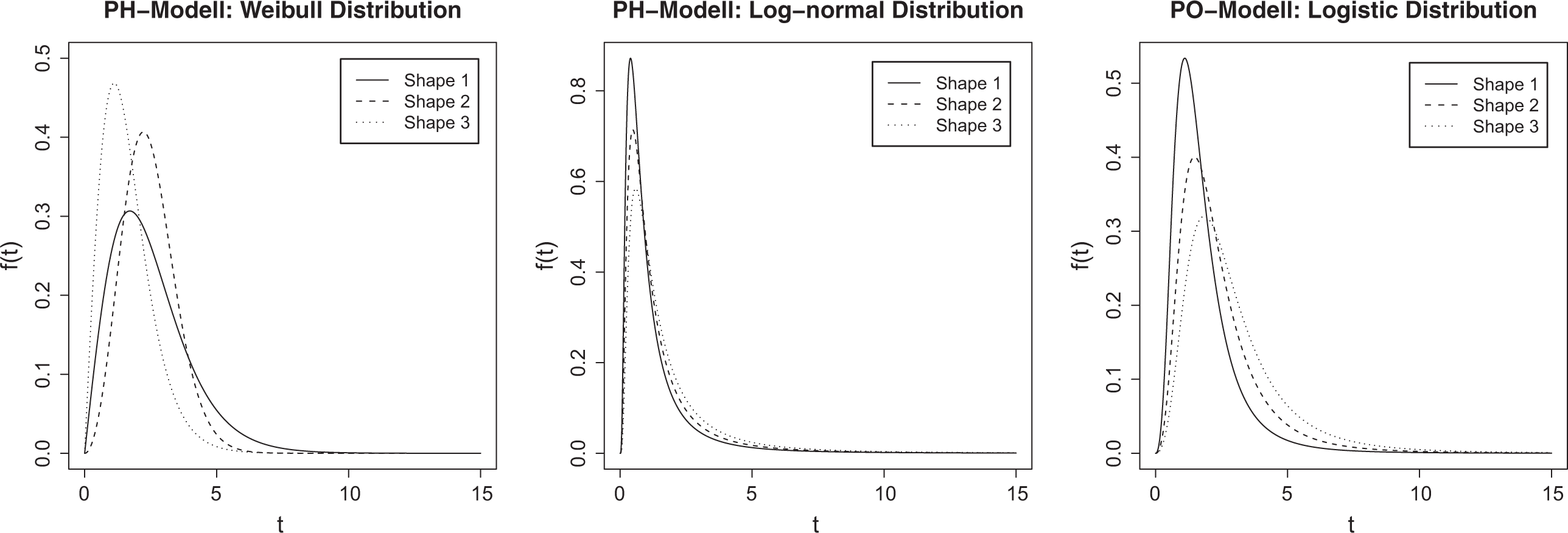
Marginal distribution of the response times in the three simulation scenarios for the three different baseline rates of information accumulation (Shape 1–Shape 3).
The proposed response time model was fit to the simulation samples by marginal maximum likelihood estimation as described previously. The integral over the normal distribution occurring in the marginal distribution of the response times (Equation 12) was approximated by Gauss-Hermite quadrature with 20 nodes. When calibrating the response time model, the response times were censored at points that roughly corresponded to the 11% and 89% quantile of the response time distribution. Between these boundaries the rate of information acquisition was modeled by a piecewise polynomial using seven segments separated at knots roughly corresponding to equally spaced quantiles. The piecewise polynomial was represented through the M-spline basis as described previously. However, for sake of comparison, additionally the rational cubic spline and the positive restricted spline were implemented. The different estimators were programmed in the statistical environment R (R Development Core Team, 2009). The scripts are available on request. Altogether, 250 simulation samples were analyzed for each simulation condition (3 Scenarios × 2 Sample Sizes). The focus of the simulation study was on parameter recovery, the recovery of the baseline rate of information acquisition and the performance of confidence intervals. The results concerning the regression coefficients and parameter τ are given in Table 1, where the true values, mean estimates, and standard errors of estimation can be found for the estimator based on the M-spline/I-spline.
Recovery of the Item Parameters in the Simulation Study for Two Sample Sizes and Three Response Time Distributions
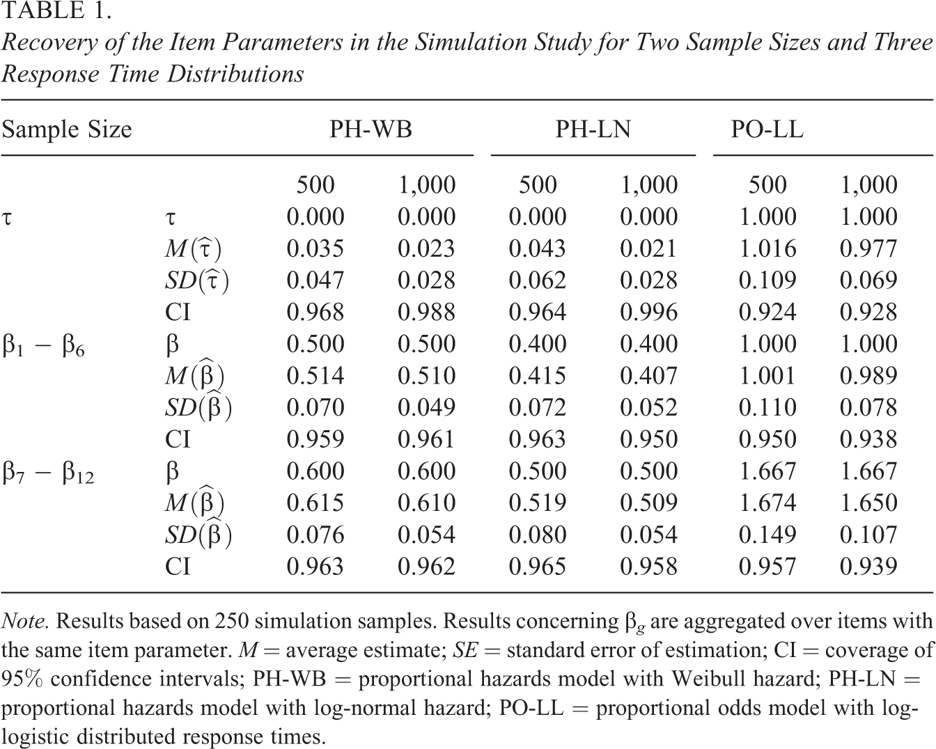
Note. Results based on 250 simulation samples. Results concerning β g are aggregated over items with the same item parameter. M = average estimate; SE = standard error of estimation; CI = coverage of 95% confidence intervals; PH-WB = proportional hazards model with Weibull hazard; PH-LN = proportional hazards model with log-normal hazard; PO-LL = proportional odds model with log-logistic distributed response times.
As can be seen, the recovery of the item parameters is generally good. In case of the proportional odds model, the parameters are unbiased. In the case of the proportional hazards models, the parameter estimates have a small bias, especially the estimate of τ. This is due to the fact that in the proportional hazards model this parameter is on the boundary of the parameter space such that its estimate does not follow a normal distribution. The coverage probability of 95% confidence intervals was good. The intervals for parameter β g seem to adhere closely to the intended coverage probability. In case of τ and the proportional hazards model, the coverage probability is too high, a fact again due to the boundary value problem. In the proportional odds model, the coverage probability seems slightly too low. However, the amount of undercoverage is small and might be beyond practical importance. When comparing the estimates from the M-splines with the estimates from the alternative approximations of the baseline rate of information acquisition little differences were found.
The recovery of the true baseline rate of information acquisition with the M-spline estimator is depicted in Figures 3 and 4 for the samples of 500 and 1,000 subjects. The figures show the true as well as the estimated baseline rates for the different scenarios. Note that in each of the three scenarios, three different baseline rates of information acquisition were employed.
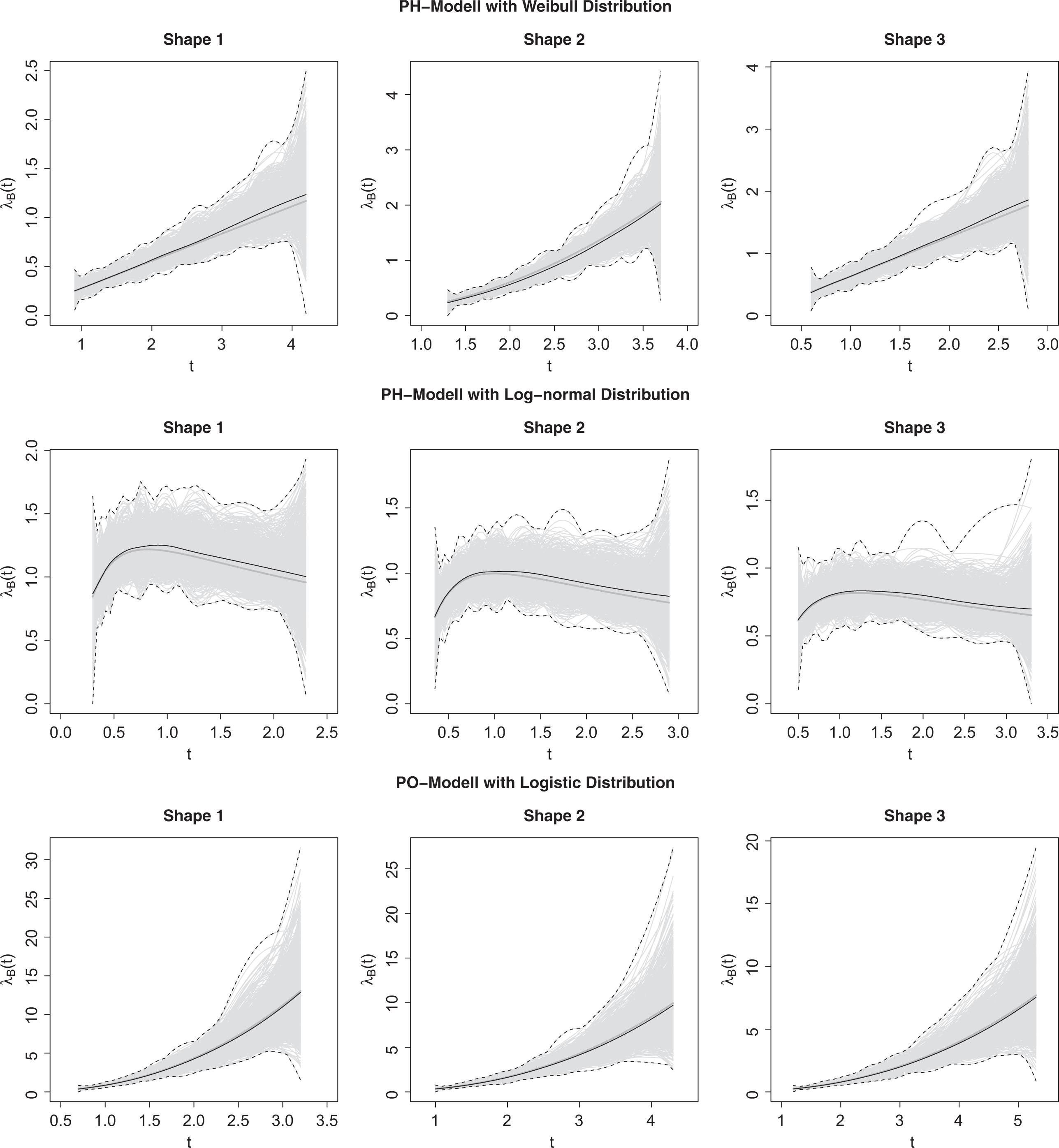
Recovery of the baseline rate of information acquisition
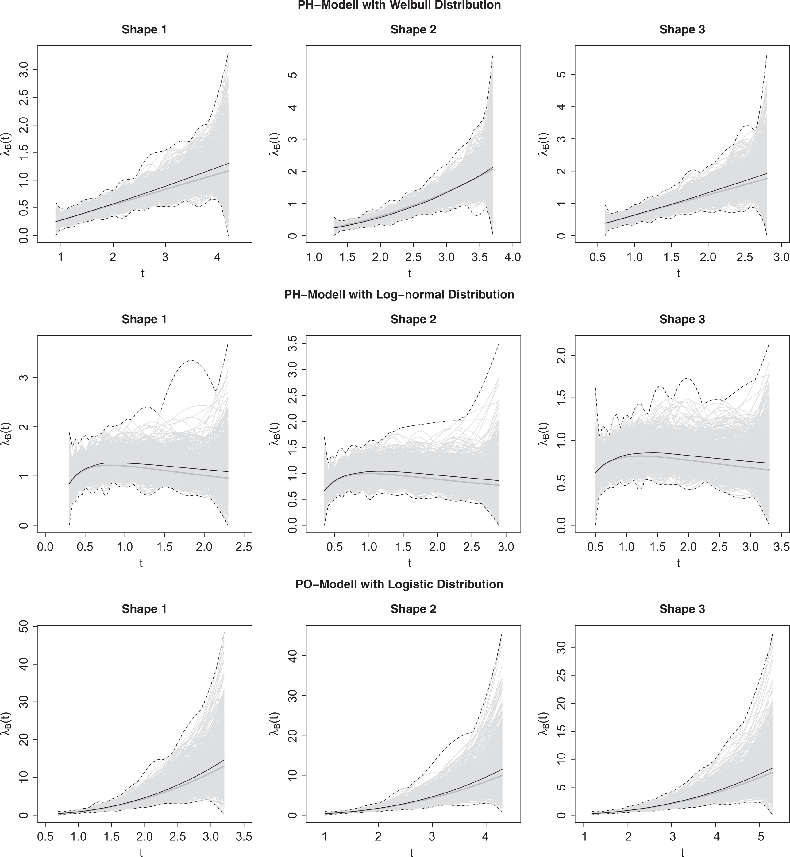
Recovery of the baseline rate of information acquisition
As can be seen, the model is flexible enough to recover the different forms of the baseline rates of information acquisition. In samples of 1,000 subjects, the true baseline rates are estimated almost without bias. However, in some samples, the single estimates deviate considerably from the true rate. Results are not that promising in samples of 500 subjects, for which the estimates are sometimes poor. So in general, rather large samples are needed in case one needs precise estimates of the baseline rate of information acquisition. When comparing the M-spline estimates with the estimates based on the alternative approximations of the baseline rate of information acquisition (positive quadratic spline and monotone quadratic rational spline), it turned out that the rational spline had a lower root mean squared error. Therefore, this approach could be an interesting alternative to the typically used M-splines.
Model Evaluation and Tests of Hypothesis
When using the proposed model for data analysis, one might need tests for several types of hypothesis: tests that evaluate the fit of the model, tests about the parameter τ, which determines the class of the model, and tests concerning the baseline rate of information acquisition. Such tests will be addressed in the following sections.
The proposed model makes assumptions about the response process that might not hold in all applications. First, the model assumes only one latent trait underlying the response times. Second, some individuals might not be comparable to the majority of the test takers as they rely on different solution strategies like rapid guessing. And third, the model presumes the same response process in correct and incorrect answers. Although the model could easily be extended by including more latent traits, allowing for different baseline rates of information acquisition in correct and incorrect responses or regarding response times in incorrect solutions as censored response times, it might be a reasonable strategy to start with the current model for the following reasons: Psychological tests are thoughtfully designed in order to measure one dominant latent trait, the majority of individuals is usually motivated to answer carefully, and modeling always requires a trade-off between model complexity and feasibility of model estimation. Nevertheless, this does not excuse someone from carefully inspecting the fit of the model. Usually, the fit of continuous latent trait models is evaluated with graphical checks like Q-Q plots and so on. However, such graphical checks can be highly misleading as they do not take the flexibility of the model into account when comparing observations and model predictions and we highly advocate the usage of additional fit tests.
The fit of the model can be assessed itemwise with a χ2-like test of goodness of fit similar in spirit to the test of Chernoff and Lehmann (1954). The test compares the observed response time distribution in each item with the response time distribution implied by the model. Therefore, the response times in an item are binned at an arbitrary number of cut points [c
0 = 0, c
1 = t
1,…, cK
= ∞]. These cut points can correspond to the knots used when approximating the baseline rate of information acquisition, but do not necessarily have to. Ideally, the cut points cover the whole range of the observed response times densely while containing enough observations at the same time. After choosing the cut points, the observed numbers of responses

whose cumulative distribution function can be approximated with a χ2 distribution according to the results given in Yuan and Bentler (2010). The degrees of freedom have to be corrected though to account for the fact that the item parameters of the model have been estimated. More details concerning the test can be found in Ranger and Kuhn (2014).
Having established the fit of the model in all items, one might want to test hypothesis about the parameter τ. In case of τ = 0, the model can be interpreted as a proportional hazards model. With τ = 1, the model is a proportional odds model. The test for the proportional hazards model therefore amounts to the test of τ = 0 versus τ > 0. In the proportional odds model, one tests τ = 1 against τ ≠ 1. The most common test of single parameter hypotheses in the maximum likelihood framework is the Wald test. This test is in fact a z-test, where the standard deviation has been determined from the information matrix. Alternatively, one could use a likelihood ratio test but would have to fit the model twice, with and without the restriction imposed by the hypothesis. Note that in case of the proportional hazards model the parameter τ is on the boundary of the parameter space. This is a violation of the regularity assumptions typically made in maximum likelihood estimation. It is well known that this invalidates the standard findings about the distribution of the parameter estimates and the likelihood ratio test statistic (Moran, 1971; Self & Liang, 1987).
Finally, it could be of theoretical importance to test hypotheses about the baseline rate of information acquisition. One might want to compare the baseline rate of different items, for example. Note that the baseline rate is modeled as a linear combination of basis functions
Simulation study—hypothesis tests
In order to evaluate the appropriateness of the proposed tests, a simulation study was conducted. Response times were generated as in the first simulation study concerning parameter recovery. That is, 2 × 3 simulation conditions were considered, which were defined by crossing two sample sizes with three response time distributions (see the previous section for more details). Having generated 250 simulation samples for each simulation condition, the item parameters were estimated as described previously, using marginal maximum likelihood estimation and censoring the response times. Then, the proposed tests were performed.
First, the test of item fit was run. Therefore, the time axis was divided into 16 time intervals at 15 time points. Then, the observed number of responses within each time interval was compared to the expected number of responses. This comparison checks whether the theoretical response time distribution and the empirical response time distribution are in agreement. For each item, the test statistic given in Equation 13 was determined as well as the corresponding p value. The results of the fit tests can be found in Table 2, where the empirical rejection rate of the tests is given for several nominal Type I error rates.
Empirical Rejection Rate of the Test for Item Fit as a Function of the Nominal Type I Error Rate α for Two Sample Sizes and Three Response Time Distributions
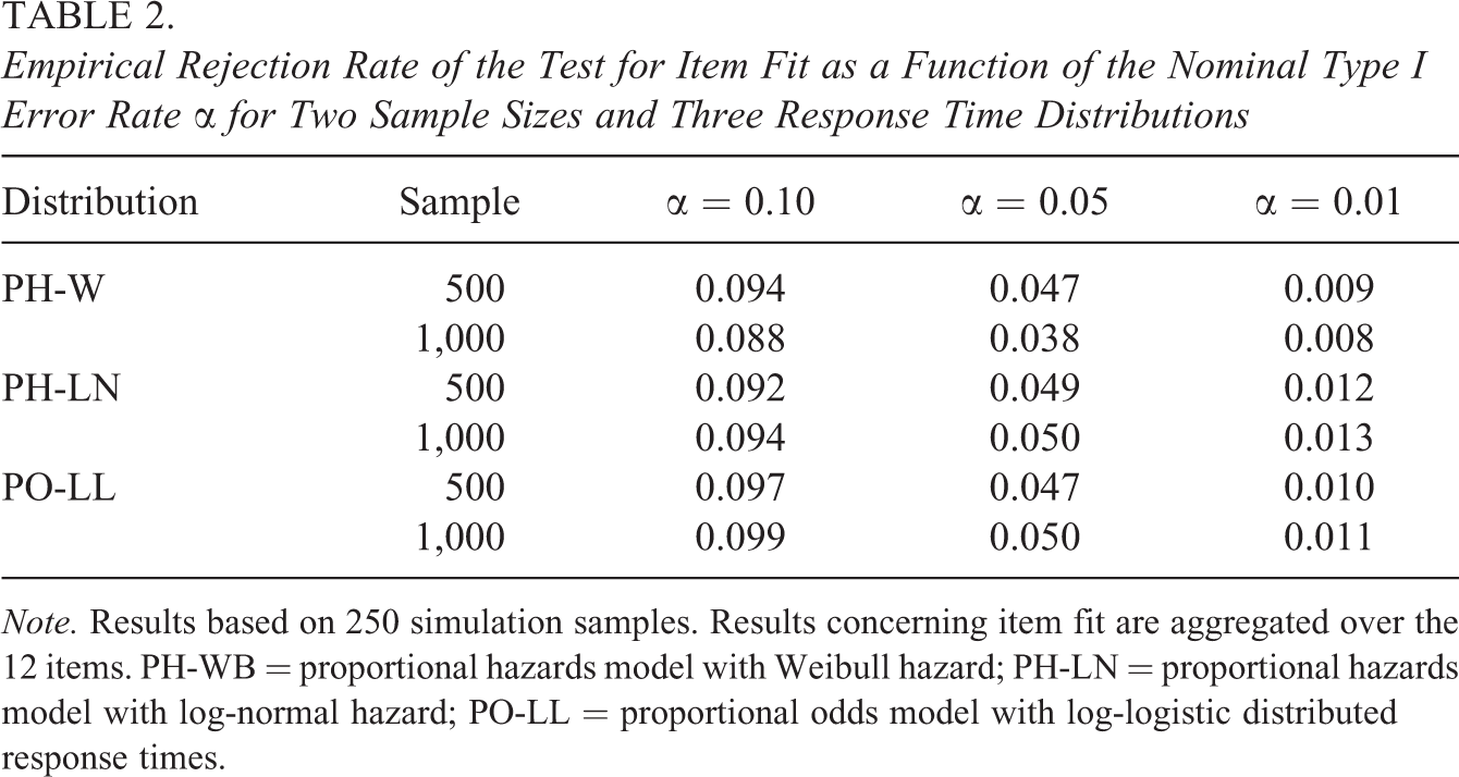
Note. Results based on 250 simulation samples. Results concerning item fit are aggregated over the 12 items. PH-WB = proportional hazards model with Weibull hazard; PH-LN = proportional hazards model with log-normal hazard; PO-LL = proportional odds model with log-logistic distributed response times.
As can be seen, the empirical rejection rates are in good agreement with the nominal Type I error rates in all conditions. This demonstrates the applicability of the test even in medium sample sizes. Note that the effect of using the same data set for model calibration and model evaluation is accounted for very well by the test.
In addition to the test of item fit, a test for specific values of τ was performed. In the proportional hazards model, the test evaluated the hypothesis of τ = 0 versus τ > 0. In the proportional odds model, the test assessed whether τ = 1 or τ ≠ 1 holds. The test was implemented as described previously, using the information matrix in order to determine the standard error of τ. Three additional tests concerning the baseline rate of information acquisition were carried out as well. The equality of the baseline rates of information acquisition was investigated for the item pairs (1,2), (3,4), (4,5), (5,6), (7,8), (9,10), and (11,12), for which this assumption was true. For the same item pairs, the hypothesis of proportional baseline rates was investigated. And finally, it was checked whether the baseline rates are shifted in these item pairs. Each such test consists of several contrasts. The constituting contrasts can be tested jointly, yielding an overall test, or separately, yielding specific tests for isolated segments of the baseline rate. Note that the basis functions are defined locally, such that the effect of one basis function is limited to a small range of the response time continuum.
The results for the tests can be found in Table 3, where the empirical rejection rates are given for several nominal Type I error rates. In samples of 500 subjects, the test for the proportionality of the baseline rates could not be calculated in 20 of the altogether 750 samples because one of the weights was extremely close to zero and the test became numerically instable.
Empirical Rejection Rate of Four Tests as a Function of the Nominal Type I Error Rate α for Two Sample Sizes and Three Response Time Distributions
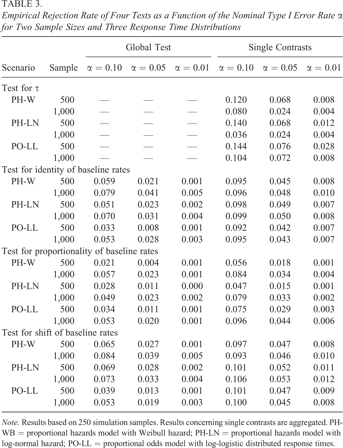
Note. Results based on 250 simulation samples. Results concerning single contrasts are aggregated. PH-WB = proportional hazards model with Weibull hazard; PH-LN = proportional hazards model with log-normal hazard; PO-LL = proportional odds model with log-logistic distributed response times.
Findings are mixed. Testing for a specific value of τ works well in the proportional odds model as long as the sample size is large enough. In the case of the proportional hazards model, the test is conservative in large samples and liberal in small. This is not totally unexpected because the asymptotic normality of maximum likelihood estimates does not hold for the boundary value τ. However, even the likelihood ratio test, which can be corrected when testing for boundary values, did not behave much better, so it seems that valid inference about τ requires rather large samples.
The tests for equality and shift of the baseline rate adhere closely to the nominal Type I error rate in case the constituting contrasts are considered separately. The global versions of the tests are rather conservative, especially in samples of 500 subjects. Their performance improves in samples of 1,000 subjects. This finding illustrates the need for large samples once more. The need for large samples is not totally unexpected. The global tests depend not only on the variances of the single contrasts but also on the whole covariance matrix and this matrix probably cannot be determined with sufficient precision in small samples. Replacing the Wald test with the likelihood ratio test might help, as the likelihood ratio test usually performs better in small samples. The test for proportionality of the hazard rate is conservative, especially in the global version when all contrasts are tested jointly. This is definitely due to the delta method as the distribution of the log contrasts deviated from the normal distribution in the smaller samples. Note that the performance of the test increases tremendously with the sample size. Again, one can speculate that likelihood ratio tests would perform better. Nevertheless, with a sample of at most 1,000 subjects the tests of the single contrasts perform sufficiently well for most purposes.
Empirical Application
In order to demonstrate the usefulness of the model, three data sets were analyzed. The first data set has already been analyzed by Ranger and Kuhn (2012) and we simply try to replicate their findings. With the second data set, we demonstrate how the rate of information acquisition can provide insights into the solution process. The third empirical example illustrates how the model can be used as a measurement model for psychological assessment.
Visual array comparison task
The first data set consisted of the response times from computer-based visual array comparison tasks. Such tests are used in the field of cognitive psychology to assess visual working memory capacity (Cowan et al., 2005; Luck & Vogel, 1997). In this test, the subjects had to remember the color of several squares that were presented together on the screen. After a blank interval, the squares were presented again. One of the squares was encircled and the subjects had to indicate whether the color of the encircled square had been changed. Overall, 48 items were used, which were administered to 1,127 children between 8 and 12 years. The data set has already been analyzed by Ranger and Kuhn (2012), who used a general linear model based on categorized response times. Here, we reanalyzed the data set and also included the test of model fit proposed previously.
The model was fit to the data as described earlier, using the M-spline for the piecewise approximation of the baseline rates of information acquisition. The segments were defined by six internal knots, located at equally spaced quantiles. Then, the model was calibrated by marginal maximum likelihood estimation. The fit of the model was assessed itemwise as described previously. Altogether, the fit of the model was excellent. Only 3 of the 48 items had a p value below α = .05 and 6 of the 48 items had a p value below α = .10. The average p value was .51. This implies that the model is capable of representing the distribution of the response times. Additionally, the fit of the model was compared with the fit of the response time model of van der Linden (2006). The response time model of van der Linden (2006) is similar to a standard factor model, but based on the log-normal distribution instead. For sake of comparability, the original model of van der Linden (2006) was extended to censored response times. Thus, the two censoring indicators were included in the likelihood and the model was estimated with marginal maximum likelihood estimation. This modification was necessary as model comparisons are only valid in cases where the data are the same for all models. Then, the information criterion of Akaike (AIC) was determined for both models (Akaike, 1992). The AIC index was 120,836.3 for the proposed model and 124,789.4 for the model of van der Linden (2006). This suggests that the proposed model provides a better approximation of the response time distribution.
The results for the regression coefficients β g were similar to the findings of Ranger and Kuhn (2012), being in a range from 0.78 to 1.52 with a mean value of 1.17. Parameter τ was estimated as 1.93, which also resembles the findings of Ranger and Kuhn (2012). Contrary to Ranger and Kuhn (2012), the rates of information acquisition were estimated in the present article. The rates of information acquisition were monotonously increasing, resembling quadratic curves. This indicates that all individuals used the same response process as mixtures of different solution strategies are indicated by nonmonotonous rates (Aalen & Gjessing, 2001).
Mental calculation test
The second data set consisted of the response times in a mental calculation test. The test contained simple addition and subtraction problems that had to be solved by second to fourth graders. Here, only the response times in the 8 items that were solved by all pupils were used. The items were generated according to the following principle. The first 2 items were single digit addition and subtraction problems without decade crossing (i.e., the result was smaller than 10; e.g., 3 + 5). The next 2 items were single digit addition and subtraction problems with a decade crossing (e.g., 6 + 7). The fifth and sixth items were two-digit problems without a decade crossing (e.g., 54 − 21). And the final 2 items were two-digit problems with a decade crossing (e.g., 34 − 18). The data set contained the responses and response times from 980 pupils.
The response time model was fit to the data set as described previously. For piecewise approximation of the baseline rate of information acquisition, the time axis was divided at six internal knots into seven segments. The choice of the knots was loosely based on the quantiles of the response time distribution; however, it was ensured that the items with the same principle of construction had the same knots. Identical knots facilitate the comparison of the baseline rate of information acquisition. Again, the M-spline was used for the approximation of the baseline rate of information acquisition. For marginal maximum likelihood estimation, the integral over the normal distribution was approximated with Gauss-Hermite quadrature using 20 nodes.
Having estimated the item parameters, the fit of the model was investigated with the proposed test. The fit was good in all items, with p values ranging from .067 to .623. This indicates that the model is capable of representing the structure of the data. A comparison with the model of van der Linden (2006) via the AIC index suggested that the proposed model (AIC = 17,312.3) fits the data better than this alternative model (AIC = 18,081.4).
The estimated baseline rates of information acquisition are depicted in Figure 5. These quantities give a more precise characterization of the response process in the calculation problems than summary statistics like the sample average or the standard deviation. Three substantive hypotheses were investigated concerning the baseline rates of information acquisition. The first test referred to the question of whether the baseline rate is identical in addition and subtraction problems that are of similar structure concerning number range and decade crossing. This hypothesis was tested for the pairs formed by the first and second item, the third and fourth item, the fifth and sixth item, and the seventh and eighth item. The second test assessed whether the rates of information acquisition are proportional in these pairs. And the third test concerned the question whether the cumulative rates of information acquisition differed by an additive constant. All tests were highly significant, except the tests in the first pair. For the first pair, the p value for identical rates was .184, the p value for proportional rates was .079, and the p value for shifted rates was .298. This indicates that the temporal course of the response process is similar in the first two problems, in contrast to the more difficult problems, where subtraction and addition appear to elicit different cognitive activity. It is plausible that pupils used fact retrieval in the first 2 items, thus relying on an identical strategy. More difficult numerical operations are usually not based on simple recall and require different solution processes (Arsalidou & Taylor, 2011).
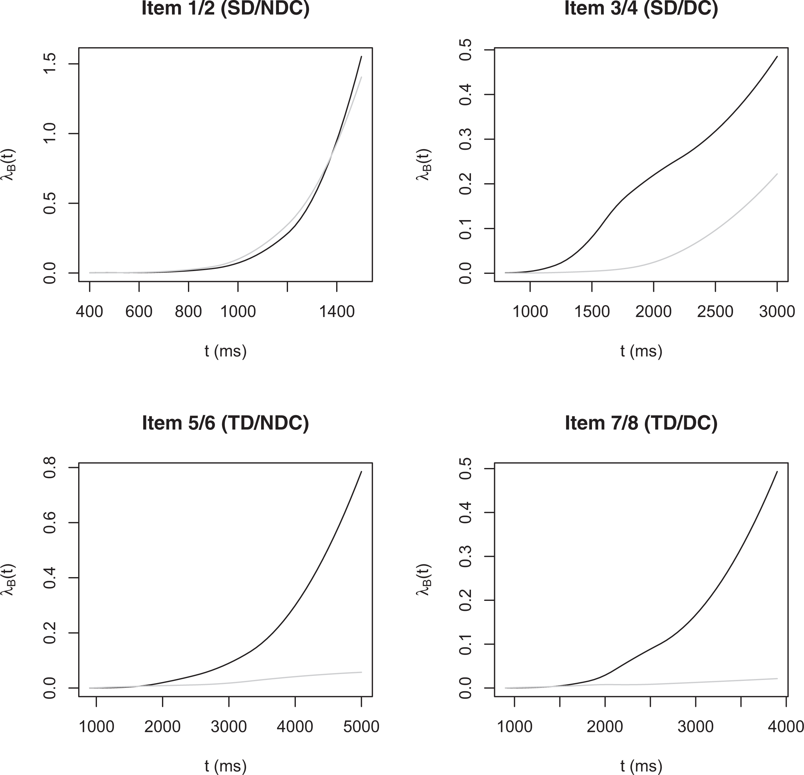
Estimated baseline rate of information accumulation for the 8 items of the mental calculation test. Items varied with respect the number of digits (SD: single-digit problem vs. TD: two-digit problem) and the need for decade crossing (DC: decade crossing vs. NDC: no decade crossing). The black line visualizes the rate in addition problems, the gray line in subtraction problems.
Chess test
In order to demonstrate the usability of the model for psychological assessment, a third data set was analyzed. This data set consisted of responses and response times in a test intended to assess chess playing proficiency. A detailed description of the test and the data can be found in van der Maas and Wagenmakers (2005). Two subscales of the test were chosen for further analysis, namely, the subscales “positional move” and “end move.” The items of the subscales contain prototypical chess problems, that is, they display a chess position, for which the best move has to be stated. In all problems, a single move is clearly superior to all other moves and therefore is regarded as the correct solution. The items from the subscale positional move refer to positional knowledge while the items from the subscale end move tap endgame knowledge. Each subscale consists of 10 items. A time limit of 30 seconds was set for each item. Overall, 259 subjects completed the test.
In a first step of data analysis, the response times in the two scales were analyzed separately with the model proposed previously. The baseline rate of information acquisition was approximated piecewisely with the M-spline, using six internal knots located at equally spaced sample quantiles. The model was calibrated with marginal maximum likelihood estimation. The fit of the model was good, although the power of the test might be low due to the small sample size. In some items, the time pressure caused by the fixed time limit was reflected in the form of the baseline rate of information accumulation, which increased sharply near the time limit. Having calibrated the model, it was used as a measurement model to estimate the latent traits of the individuals, regarding the estimated item parameters as the true ones. The traits were determined with the expected a posteriori estimator, which is the conditional expectation of the latent trait when conditioning on the observed response times of an individual. In addition to the proposed model, three alternative models were fitted to the data, namely, a standard factor model for the logarithmized response times, a modified version of the model of van der Linden (2006) for censored response times, and a Rasch model for the responses. These three models were used as measurement models too.
As an external criterion of chess playing proficiency the data set contains the so-called Elo-score of each chess player, which is an index formed by his or her past success when playing chess. The Elo-score can be considered as an excellent proxy of the true chess playing proficiency of a test taker. In order to assess the diagnostic utility of the model and the latent trait estimates, we investigated the incremental validity that can be achieved when using the response times in addition to the responses alone. Therefore, we predicted the Elo-scores with a linear regression model, in which the different trait estimates were entered. With the estimated latent traits from the Rasch model, the Elo-score could be predicted with R 2 = .443 in the positional move scale and with R 2 = .440 in the end move scale. Using the trait estimates from the Rasch model and the overall time of an individual, the Elo-score could be predicted with R 2 = .474 in the positional move scale and with R 2 = .456 in the end move scale. Using the trait estimates from the Rasch model and trait estimates from the factor model, the Elo-score could be predicted with R 2 = .498 in the positional move scale and with R 2 = .484 in the end move scale. With the estimates from the Rasch model and the model of van der Linden (2007), the predictive validities were R 2 = .488 in the positional move scale and R 2 = .474 in the end move scale. The highest validity could be achieved with the estimates from the Rasch model and the estimates from the current model, by which the Elo-score could be predicted with R 2 = .501 in the positional move scale and with R 2 = .486 in the end move scale. Using interaction terms of the latent traits did not improve the external validity much.
This study demonstrates two findings. First, the external validity of a test can be increased by using the response time data provided by the test takers. And second, it is beneficial to use a response time model. The proposed model achieved the highest incremental validity although the difference to the log-normal model or the model of van der Linden (2006) is negligible and the traits of the two models were more or less exchangeable. Note that the predictive performance of the proposed model could even be higher had the response times not been censored. This at least suggests the comparison between the log-normal model and the modified model of van der Linden (2006) that largely differ in the fact that the response times were censored in one model but not in the other.
Discussion
A typical finding for response time data in achievement tests is the observation that individuals differ systematically in their speed of working when trying to solve the items. This observation raises the question of how to model these individual differences in work pace. This is far from clear as there are two different conceptualizations concerning the work pace of an individual. In the first one, the increased speed of some test takers is due to an increase of their processing capacity, achieved by allocating more resources of the information processing system to a task. This is similar to the change from a 32-bit computer to a 64-bit computer. This view of work pace leads to the proportional hazards model, popular in survival time analysis but also applicable in experimental psychology (Wenger & Gibson, 2004). Alternatively, one could think that an individual accelerates the single process steps, similar to overclocking the central processing unit of a computer. The resulting model is the accelerated failure time model, where the time axis is shrunk or stretched according to an acceleration factor. The mathematical core of accelerated failure time models consists in the decomposition of the log response times into a systematic part depending on predictors and an error term of unknown distribution. Both approaches can be subsumed into a common framework, the linear transformation model.
In the present article, we have proposed a model that subsumes particular representatives of the linear transformation model. As shown previously, the model has an attractive interpretation in terms of an information accumulation process. Thereby, the transformation of the response times, which is usually considered as a nuisance parameter complicating model estimation, receives a psychological interpretation. This interpretation however is not crucial for an application of the model in case one questions the utility of cognitive process models for test response times. In case one disagrees about the accumulator interpretation, one can simply consider the model as a flexible approach to response time modeling that subsumes several standard models. In this respect, it is similar to the Box-Cox normal model of Klein Entink, van der Linden, and Fox (2009).
Model calibration and model inference can be accomplished within the framework provided by marginal maximum likelihood estimation. The proposed methods work generally well, although in the case of the proportional hazards model some tests are too conservative and rather large samples are needed for model calibration and valid inference. Some tests concerning the form of the baseline rate of information acquisition were described in the article. But of course, there are more hypotheses one could investigate. Testing the baseline rate of information acquisition for special forms like concavity or bimodality might be of theoretical importance. Unfortunately, such tests have not been developed so far. This is definitely a topic for future research.
The proposed model should be seen as a tool in response and response time modeling. It can be used as a measurement model in order to estimate the latent work pace of individuals. It can also be used as a diagnostic tool in order to analyze the response process. Measurement invariance, for example, might be a field where it should be interesting to have a more detailed picture of the information accumulation process. In the present article, we only considered response times focusing on the speed of information processing. The responses were ignored. However, the actual model can be extended to a joint model for responses and response times in order to assess the speed and accuracy of the information processing capabilities of an individual (Davison, Semmes, Huang, & Close, 2012). One approach to a joint model is provided by the hierarchical framework of van der Linden (2007) that postulates separate models for responses and response times which are related on a second level. The proposed response time model can simply be integrated into this framework by replacing the original response time model of van der Linden (2007). Alternatively, in cases where one considers correct and incorrect responses as resulting from different response processes, one could model the response times conditionally on the responses. That is, one could assume different baseline rates of information acquisition for different responses. Such an approach, combined with a standard item response model for the responses, also yields a joint model for the responses and the response times of a test. In the present article, we only indicated some of the potential uses and extensions of the model. Nevertheless, we hope that the model will prove to be useful in test development and psychological assessment.
Footnotes
Acknowledgments
We would like to thank the Editor, Dr. Sinharay, and three referees for their helpful and constructive comments, which led to many improvements. We are also indebted to H. van der Maas and E. Wagenmakers for the permission to use the Amsterdam Chess Data.
Declaration of Conflicting Interests
The author(s) declared no potential conflicts of interest with respect to the research, authorship, and/or publication of this article.
Funding
The author(s) disclosed receipt of the following financial support for the research, authorship, and/or publication of this article: The second author of this article was supported by a grant of the German Federal Ministry of Education and Research (grant no. 01GJ1006).