Improving Estimation for Two-Dimensional Regression Discontinuity Designs in Education With Gaussian Process Regression

Abstract

Sometimes a treatment, such as receiving a high school diploma, is assigned to students if their scores on two inputs (e.g., math and English test scores) are above established cutoffs. This forms a multidimensional regression discontinuity design (RDD) where there are two running variables instead of one. Present methods for estimating such designs either collapse the two running variables into a single running variable, estimate two separate one-dimensional RDDs, or jointly model the entire response surface. The first two approaches may lose valuable information, while the third approach can be very sensitive to model misspecification. We examine an alternative approach, developed in the context of geographic RDDs, which uses Gaussian processes to flexibly model the response surfaces and estimate the impact of treatment along the full range of students who were on the margin of receiving treatment. We also discuss parametric and nonparametric surface response methods in general, which have been under explored in multidimensional RDDs for education. We demonstrate theoretically, in simulation, and in an applied example, that the Gaussian process approach has several advantages over current approaches, including other surface response methods. In particular, using Gaussian process regression in two-dimensional RDDs shows strong coverage and standard error estimation and allows for easy examination of treatment effect variation for students with different patterns of running variables and outcomes. As nonparametric approaches are new in education-specific RDDs, we also provide an R package for users to estimate treatment effects using these methods.

Keywords

nonparametric methods regression discontinuity design surface response Gaussian process

1. Introduction

Regression discontinuity designs (RDDs) were first introduced by Thistlethwaite and Campbell (1960) and are widely used in economics, education, political science, and statistics for estimating causal effects. In a classical RDD, treatment assignment is determined by a single covariate, called a “running variable,” being above or below a cutoff. The goal of an RDD is to estimate the causal effect of treatment on outcomes while accounting for the discontinuous nature of treatment assignment, such as the effect of education grants provided to families with incomes below a certain threshold (Li et al., 2015; Ludwig & Miller, 2007).

RDDs are valuable because, even though treatment assignment is completely confounded by the running variable, the causal effect at the cutoff is identifiable under the mild assumption that the treatment and control outcomes are continuous around the cutoff (J. Hahn et al., 2001). Many have utilized nonparametric approaches—in particular, local linear regression methods that upweight subjects near the cutoff—to model the data above and below the cutoff (Cattaneo & Titiunik, 2022; Imbens & Lemieux, 2008; Pei et al., 2022). The causal effect can then be estimated as the difference between the extrapolations of these regressions to the cutoff.

We focus on the case of RDDs, which have more than one running variable. For example, often in education applications, treatment—such as access to a tutoring program or a high school diploma—is assigned to students based on multiple test scores, for example, whether or not a student passed both a math and an English test (Ou, 2010; Papay et al., 2014; Reardon et al., 2010). This is similar to geographic RDDs, where treatment is assigned based on units’ latitude and longitude locations, which act as the running variables (L. Keele et al., 2015; L. J. Keele & Titiunik, 2015; Rischard et al., 2021). We focus throughout on RDDs that use two running variables to estimate the effect of only one treatment. In this setting, the cutoffs on the two running variables in a two-dimensional RDD form a boundary within a two-dimensional space, where units are treated on one side of the boundary, but not the other. While the causal estimand in a one-dimensional RDD is the average treatment effect at the cutoff, the causal estimand in a two-dimensional RDD is the average treatment effect along the boundary, which may vary across different boundary points. These location-specific treatment effects are often aggregated into a single measure using researcher-specified weights. The resulting aggregate measure is called a boundary average treatment effect (BATE).

Estimating these causal estimands is not as straightforward as estimating an average treatment effect at the cutoff point in the one-dimensional case using local linear regression. Several common methods attempt to estimate causal effects in a two-dimensional RDD by extending methods for the one-dimensional case, but these are limited in that they only target an aggregate BATE estimand that may lack interpretability. For example, one method collapses the two running variables into a single running variable and then follows standard local linear regression methods (Cohodes & Goodman, 2012; Martorell, 2005; Robinson, 2011), while another estimates two separate one-dimensional RDDs for each running variable (Kane, 2003; Papay et al., 2010; Reardon et al., 2010). These approaches, though straightforward extensions of existing methods, reduce the problem to one dimension: This not only loses valuable information but also does not target location-specific treatment effects along the boundary by only targeting an aggregate estimand (see Rischard et al., 2021 for further discussion). Response surface modeling methods have also been used to estimate two-dimensional RDD causal effects; while this allows one to estimate location-specific treatment effects, they can be sensitive to model specification when conducted parametrically (Dee, 2012; Papay et al., 2011, 2014).

Given these challenges, using existing methods for estimating average causal effects in two-dimensional RDDs, we propose using a nonparametric surface response modeling approach. This has several advantages over current approaches, namely that it flexibly estimates the mean outcome on both sides of the boundary. This makes model misspecification less of a concern. Uniquely, this approach also allows for easy examination of treatment effect variation along the boundary, in addition to aggregate BATE estimands. We compare current two-dimensional RDD approaches, including parametric surface response, to nonparametric surface response methods that use Gaussian process regression and locally weighted regression (loess).

We make four main contributions to the literature. First, we demonstrate how this Gaussian process regression (GPR) approach can be used to flexibly estimate treatment effects along the boundary in two-dimensional RDDs in education, as well as aggregated causal effects. Second, we discuss surface response methods in general, which seem to have been underexplored in the literature. For example, we also discuss a loess-based approach that we believe has not been explored in the literature but is easy to implement. Third, we conduct a simulation study to compare methods that reduce the two-dimensional RDD down to one dimension to surface response methods that utilize the two-dimensional context in which these RDDs occur. Finally, we provide the R package, twodrdd, to implement our approach.

In Section 2, we define the notation, setup, and causal estimands for two-dimensional RDDs. In Section 3, we review current methods for analyzing two-dimensional RDDs, and in Section 4, we present competing parametric and nonparametric surface response approaches. In Section 5, we describe the Gaussian process regression approach, and in Section 6, we discuss a straightforward loess-based approach, which we believe has not been previously studied for multidimensional RDDs. In Section 7, we compare these various methods via simulation, and we find that Gaussian process regression shows better performance in terms of bias, standard errors, and root mean square error (RMSE), in addition to much stronger coverage of treatment effects and estimation of standard errors. We further demonstrate these methods in Section 8 by analyzing an educational policy test-score cutoff in Wisconsin. Here, we show how using Gaussian process regression can help illuminate patterns of treatment effect heterogeneity for differently scoring students, as well as provide more precise inference over prior analyses that use one-dimensional approaches. Finally, we conclude in Section 9.

2. Notation, Setup, and Causal Estimands

Consider $N$ units, indexed by $i$ , each with treatment assignment $W_{i}$ , outcome $Y_{i}$ , and running variables $X_{1 i}$ and $X_{2 i}$ . We focus on sharp two-dimensional RDDs, where

\begin{matrix} W_{i} = {\begin{matrix} 1 & if X_{1 i} \geq c_{1} and X_{2 i} \geq c_{2} \\ 0 & otherwise . \end{matrix} \end{matrix}

(1)

for fixed, scalar cutoffs $c_{1}$ and $c_{2}$ . This design requires that the individual receive one treatment on the basis of passing two score cutoff thresholds, and receive no treatment otherwise. For example, $X_{1}$ and X₂ might be math and reading scores, and the cutoffs represent eligibility to receive a high school diploma, such as with high school exit examinations. The outcome might be eventual college enrollment. Other policy designs may allow for different treatments if only one of the score cutoffs were met, but we do not focus on those here.

Let $Y_{i}$ (1) and $Y_{i}$ (0) denote the potential outcomes of the unit $i$ under treatment $W_{i} = 1$ and control $W_{i} = 0$ , respectively. The observed outcomes can then be written as a function of the potential outcomes: $Y_{i} = W_{i} Y_{i} (1) + (1 - W_{i}) Y_{i} (0)$ . The outcome $Y_{i} (1)$ is observed only if the unit $i$ is exposed to treatment ( $W_{i} = 1$ ), and $Y_{i} (0)$ is only observed if the unit $i$ is not exposed to treatment ( $W_{i} = 0$ ).

In sharp RDDs, the probability of receiving treatment for every unit is 0 or 1. There are also fuzzy RDDs, where the probability of receiving treatment at the threshold still changes, but can change by a smaller jump (see Imbens and Lemieux (2008) for a conceptual review of sharp and fuzzy RDDs). We focus on sharp RDDs because they are particularly common in education applications, where students gain access to a program or treatment if and only if two test scores fall to one side of their given cutoffs.

Figure 1 plots an example of this type of RDD. The data for this figure come from our applied example using Wisconsin student test scores (the two running variables) from students who are English language learners (ELLs). Treatment is reclassification into non-ELL status, and the outcomes we observe are students’ ACT college admissions test scores. This reclassification involves a change in students’ educational experience in schools, where formerly ELL students join “mainstream” non-ELL classrooms and lose access to ELL-specific supports. The cutoffs in this RDD are the solid $c_{1} = 0$ and $c_{2} = 0$ black lines, the treated units in the top right quadrant are colored in dark blue, and the control units are colored in light blue.

Figure 1.

An example of the two-dimensional RDD we consider in this paper. The cutoffs are the solid black lines $c_{1} = 0$ along running variable 1 and $c_{2} = 0$ along running variable 2. The dark blue treated region is in the top right quadrant, and the light blue control region is the region to the left and below the boundary defined by the cutoffs.

Other common applications in education assign treatment, such as access to summer school, if the student performs poorly on either test, which would change the inequalities in Equation 1 to an $or$ statement between running variable values that were less than the cutoffs. This setup was the focus of a simulation study in Porter et al. (2017) that compared various methods for analyzing two-dimensional RDDs, where their control units were in the top right quadrant and treated units were in the remaining three quadrants. That study simulated 5,000 data points from a standard two-dimensional normal distribution with varying correlations between the two running variables, and we revisit this study design in Section 7.

2.1. Causal Estimand

Unlike a one-dimensional RDD where the causal estimand is the average treatment effect at a single cutoff value, the causal estimand in this two-dimensional RDD depends on the boundary created by the two cutoffs (colored in black in Figure 1). While geographic RDDs use irregular boundaries, two-dimensional RDD applications in education typically use test score cutoffs or other running variable cutoffs that are single values. Our focus in this article is therefore on a rectangular boundary.

The causal estimand is the average treatment effect at individual locations along the boundary, which can then be aggregated into an overall causal estimand. To formalize these causal estimands, define the boundary as

\begin{matrix} B = {x : x_{1} = c_{1} and x_{2} \geq c_{2}, or x_{2} = c_{2} and x_{1} \geq c_{1}}, \end{matrix}

(2)

where $x = (x_{1}, x_{2})$ is some realization of the two running variables. Then, we use $τ (x)$ to denote the average treatment effect at a particular boundary point $x \in B$ ; this is defined as

\begin{matrix} τ (x) = E [Y_{i} (1) - Y_{i} (0) | X_{1 i} = x_{1}, X_{2 i} = x_{2}], \end{matrix}

(3)

where $x \in B$ .

Throughout, we assume that these conditional expectations are continuous at $x \in B$ , which is needed to identify $τ (x)$ . These location-specific treatment effects $τ (x)$ are then often aggregated into a single BATE using weights $w (x)$ :

τ^{w} = \frac{\int_{x \in B} w (x) τ (x) d x}{\int_{x \in B} w (x) d x} .

(4)

We denote the BATE as $τ^{w}$ to emphasize its dependence on the choice of weight function $w (x)$ , which has to be determined by the researcher.

The simplest form of weights are uniform weights, defined as $w (x) = 1$ , which place equal weight on every point along the boundary. However, this is usually not a sensible choice if there is little data along some parts of the boundary, such as at the center-top or far-right portions of the boundary in Figure 1.

Following this logic, researchers often place more weight on sections of the boundary with denser populations of units, that is, setting $w (x) = ρ (x)$ , where $ρ (x)$ is the density of units at $x$ . This defines the following causal estimand:

τ^{pop} = \frac{\int_{x \in B} ρ (x) τ (x) d x}{\int_{x \in B} ρ (x) d x} .

(5)

Such weights have previously been considered by Porter et al. (2017) and Wong et al. (2013). A benefit of this estimand is that it, in principle, corresponds to the average treatment effect of the super-population of units residing on the boundary (Imbens & Zajonc, 2011; Keele & Titiunik, 2015; Rischard et al., 2021). In practice, $ρ (x)$ must be estimated, such as by using a kernel density estimator.

We can also estimate averages over portions of the boundary. In particular, in Figure 1, we can separately estimate the average treatment effect for the vertical boundary (where the running variable $X_{1}$ is fixed) and a horizontal boundary (where $X_{2}$ is fixed). Define $B_{1} = {x : x_{1} = c_{1}, x_{2} \geq c_{2}}$ and $B_{2} = {x : x_{1} \geq c_{1}, x_{2} = c_{2}}$ as these sections of the boundary. Then, we have the following causal estimands:

\begin{array}{l} τ_{1}^{w} = \frac{\int_{x \in ℬ_{1}} w (x) τ (x) d x}{\int_{x \in ℬ_{1}} w (x) d x}, \\ τ_{2}^{w} = \frac{\int_{x \in ℬ_{2}} w (x) τ (x) d x}{\int_{x \in ℬ_{2}} w (x) d x} . \end{array}

(6)

We also have that the overall BATE is then a weighted average of the two sub-BATEs:

τ^{w} = W_{1} τ_{1}^{w} + (1 - W_{1}) τ_{2}^{w},

where $W_{1}$ is the relative weight $W_{1} = \int_{x \in B_{1}} w (x) d x / (\int_{x \in B_{1}} w (x) d x + \int_{x \in B_{2}} w (x) d x)$ .

There are good reasons we might focus on $τ_{1}^{w}$ and $τ_{2}^{w}$ over $τ^{w}$ . Wong et al. (2013) discusses how, under the density approach, simply scaling a running variable $d$ will change the corresponding edge weight $W_{d}$ . The BATE is then not as well-defined a quantity as we might believe. Given this, Wong et al. (2013) advocate for focusing on the edge-specific estimands, which are stable to arbitrary linear scalings. To mitigate these concerns, we advocate for standardizing the running variables or using precision weights (discussed in Section 5.4) and, more importantly, for examining the estimate of the full function $τ (x)$ , as we illustrate in the empirical section. We discuss scaling further in Supplemental Appendix Section 10.2.

Note that $τ_{1}^{w}$ and $τ_{2}^{w}$ in Equation 6 are special cases of $τ^{w}$ in Equation 4, where for $τ_{1}^{w}$ we have set $w (x) = 0$ for $x \in B_{2}$ , and likewise for $τ_{2}^{w}$ we have set $w (x) = 0$ for $x \in B_{1}$ . However, the causal estimands in the two-dimensional RDD literature are usually not written in the form of Equation 6. More typically, they are written in the following form

\begin{matrix} τ_{1} = E [Y_{i} (1) - Y_{i} (0) | X_{1 i} = c_{1}, X_{2 i} \geq c_{2}], τ_{2} = E [Y_{i} (1) - Y_{i} (0) | X_{2 i} = c_{2}, X_{1 i} \geq c_{1}] . \end{matrix}

(7)

For examples of this form for the causal estimands, see Porter et al. (2017), Equations 1 and 2, as well as the 13 papers they discuss in their literature review of two-dimensional RDDs. We prefer the form of Equations 6 over 7 for defining these causal estimands because it is more flexible and more explicit. It is more flexible because it defines a large class of weighted average treatment effects that may be of interest depending on the application, and it is more explicit because it makes clear what kind of “averaging” is being done across the boundary. Meanwhile, the expectation in Equation 7 is usually with respect to some hypothetical infinite population, meaning that it is (implicitly) using population-density weights to define a BATE.

2.2. Identification Assumptions

We note that identification of these causal estimands for multidimensional RDDs must meet RDD assumptions similar to those in one dimension. In our setting, we are examining one treatment that is assigned on the basis of two score cutoffs. Therefore, there must be a discontinuity in the probability of treatment at the boundary formed by the cutoff scores. Additionally, there must be continuity of potential outcomes at the boundary, and the inability of individuals to sort above or below the cutoff (e.g., by manipulating the value of their running variables). For further discussion of these assumptions, see Reardon and Robinson (2012) and Wong et al. (2013).

3. Local Linear Regression-Based Approaches for Two-Dimensional RDDs

In this section, we review state-of-the-art methods for analyzing two-dimensional RDDs. As most current RDD methods leverage local linear regression approaches, we first review local linear regression for one-dimensional RDDs, and then turn to two-dimensional RDD estimation.

3.1. Using Local Linear Regression for One-Dimensional RDDs

Consider the case where there is only one running variable $X$ with cutoff $c$ , and define treatment as $W_{i} = 1$ if $X_{i} \geq c$ and 0 otherwise. In this case, the causal estimand is the average treatment effect at the cutoff, defined as

\begin{matrix} τ (c) = E [Y_{i} (1) | X_{i} = c] - E [Y_{i} (0) | X_{i} = c] \end{matrix}

(8)

As noted in J. Hahn et al. (2001), “any nonparametric estimator [can be used] to estimate” $E [Y_{i} (1) | X_{i} = c]$ and $E [Y_{i} (0) | X_{i} = c]$ . Local linear regression is a popular method for analyzing one-dimensional RDDs because of its desirable boundary properties (Cattaneo & Titiunik, 2022; Imbens & Lemieux, 2008; J. Hahn et al., 2001). Researchers such as Calonico et al. (2014, 2018) have used bias corrections to improve local linear regression methods, and this approach has become popular in econometrics (Athey & Imbens, 2017).

There are also alternatives to local linear regression. The local randomization literature (Branson & Mealli, 2018; Cattaneo et al., 2015; Li et al., 2015; Sekhon & Titiunik, 2017) envisions the RDD as an as-if randomized experiment around the cutoff, due to randomness in the running variable. In this setup, they estimate the average treatment effect in a neighborhood of the cutoff by assuming assignment is unconfounded given observed covariates. Cattaneo et al. (2017) compare local randomization methods to local linear regression methods, and Díaz and Zubizarreta (2023) consider local randomization for complex RDDs with multiple treatment assignment rules.

Finally, there are Bayesian approaches to RDDs (Alcantara et al., 2024; Chib & Jacobi, 2016; Chib et al., 2023; Geneletti et al., 2015; Li et al., 2015). Branson et al. (2019) proposed using Gaussian process regression to analyze one-dimensional RDDs and found that this approach exhibited promising coverage, interval length, and mean squared error over local linear regression methods. Following Rischard et al. (2021), we propose the use of Gaussian process regression for two-dimensional education RDDs in Section 5, but first, we review other current approaches for analyzing two-dimensional RDDs.

3.2. Current Approaches for Analyzing Two-Dimensional RDDs

There are three leading methods in the literature for analyzing sharp two-dimensional RDDs like those presented in Figure 1. Porter et al. (2017) and Wong et al. (2013) reviewed them and conducted simulation studies comparing methods. The three methods described below attempt to simplify the two-dimensional RDD into a one-dimensional RDD so that local linear regression methods can be used. We discuss their implementation in the Supplemental Appendix Section 10.1. In Section 4, we discuss surface response methods, which more explicitly acknowledge the two-dimensional nature of these RDDs without simplifying them to one-dimensional RDDs:

The binding score method: This method reduces the two-dimensional RDD into a unidimensional problem. It uses both running variables to define a “binding score” under the rationale that one score (either the minimum or maximum of the running variables for each unit) will be responsible for a unit’s assignment to treatment by falling either above or below the cutoff. The binding score then acts as the running variable in a one-dimensional RDD that uses local linear regression. In the case of Figure 1, where units receive treatment only if both running variables meet the threshold, the binding score $B S_{i}$ is defined as $\min (X_{1 i}, X_{2 i})$ after $X_{1 i}$ and $X_{2 i}$ are centered around their cutoffs. This method implicitly makes the assumption that $τ_{1} = τ_{2}$ , defined in Equation 7, and will target some weighted average of $τ_{1}$ and $τ_{2}$ if they differ. This method has been discussed in works such as Cohodes and Goodman (2012), Martorell (2005), and Robinson (2011).

The frontier method and pooled frontier: The frontier method divides a two-dimensional RDD into two one-dimensional RDDs using standard approaches (e.g., local linear regression described in Section 3.1). First, units that are not assigned to treatment because of the values of both running variables are discarded, which may decrease precision due to a smaller sample size. For example, the units in the lower-left quadrant of Figure 1 would be discarded because $X_{1 i} < c_{1}$ and $X_{2 i} < c_{2}$ . Then, once the running variables are centered around their cutoffs, the upper quadrants of Figure 1 can be viewed as a one-dimensional RDD across the boundary defined by $c_{1} = 0$ , where treatment is determined only by $X_{1}$ with $X_{2}$ being a nuisance variable. Similarly, only $X_{2}$ determines treatment across the $c_{2} = 0$ boundary in the right-hand quadrants and $X_{1}$ is a nuisance variable. This method’s two one-dimensional RDD analyses provide estimates for $τ_{1}$ and $τ_{2}$ in Equation 7. The frontier approach has been discussed in works such as Kane (2003), Papay et al. (2010), and Reardon et al. (2010). The pooled frontier method extends the frontier by estimating the BATE per Equation 4 as a weighted average of the estimated treatment effects on both segments of the boundary, using the proportion of data close to each arm of the boundary as the weights (see Wong et al., 2013, Equations 3–5). As a result, observations near the intersection above the treatment cutoff boundary segments are incorporated twice into the BATE estimate. Furthermore, while each estimated component is well defined by the one-dimensional RDD, the relative weights of the two components depend on the relative total density along the components, which is sensitive to the scaling of the running variable. In particular, as one scales one running variable higher and higher, it will receive more and more weight; if there is heterogeneity, this can shift the BATE; see Wong et al. (2013) for an extended discussion of this issue. They therefore argue to look at each boundary individually, rather than pooling them. Porter et al. (2017), who also focused on $τ_{1}$ and $τ_{2}$ separately, recommend using the frontier method in most situations due to its strong performance and straightforward implementation in their simulation study. However, they did recommend comparing it to the binding score method if there is reason to believe that average treatment effects are similar along both segments of the boundary.

The fuzzy instrumental variable method: Like the frontier method, this method generates two separate one-dimensional RDD estimates, but it does so while using more sample data. By viewing Figure 1 as a one-dimensional RDD in terms of $X_{1}$ (and thus ignoring $X_{2}$ ), there is non-compliance to the right of $c_{1}$ because some units receive the control condition even though they are on the treated side. This can therefore be viewed as a fuzzy one-dimensional RDD. Fuzzy RDDs can be estimated by defining an instrumental variable (IV) for treatment assignment and targeting a local average treatment effect among compliers at the boundary for $X_{1}$ and, separately, $X_{2}$ (Imbens & Lemieux, 2008). The IV approach requires additional assumptions of continuity in the conditional expectation of the treatment assignment at the boundary, as well as monotonicity (that treatment is non-increasing at the boundary). These assumptions are often difficult or impossible to test in practice, and violations can introduce bias. This method has been discussed in works such as Dee (2012), Robinson (2011), and Wong et al. (2013). Porter et al. (2017) found this method to more frequently exhibit bias and have higher variance than others, and we therefore do not investigate it.

4. Surface Response Approaches

Surface response approaches, in contrast, view the two-dimensional RDD as, indeed, a two-dimensional RDD, instead of simplifying the problem into one-dimensional RDDs. This means that they are able to target the overall treatment effect $τ^{w}$ while local linear regression-based methods conduct inference for the estimands $τ_{1}^{w}$ and $τ_{2}^{w}$ . Furthermore, surface response approaches estimate the location-specific treatment effects $τ (x)$ , which allow one to measure possible treatment effect heterogeneity along the boundary.

Specifically, the surface response approach models the mean potential outcome regression functions $μ_{T} (X_{1 i}, X_{2 i}) = E [Y_{i} (1) | X_{1 i}, X_{2 i}]$ and $μ_{C} (X_{1 i}, X_{2 i}) = E [Y_{i} (0) | X_{1 i}, X_{2 i}]$ for treatment and control, respectively, which results in a three-dimensional surface. The surface response approach models treatment effects as discontinuities in the surfaces between the treatment and control groups while still requiring the identifying assumptions, such as continuity of the mean potential outcomes at the boundary and the existence of a discontinuity in treatment probabilities at the boundary. There are two ways to estimate $μ_{T} (X_{1 i}, X_{2 i})$ and $μ_{C} (X_{1 i}, X_{2 i})$ : parametrically and nonparametrically.

As an example of a parametric surface response approach, Equation 9 gives a linear surface response model:

\begin{matrix} Y_{i} = α + τ W_{i} + β_{1} X_{1 i} + β_{2} X_{2 i} \\ + δ_{1} (X_{1 i} \times W_{i}) + δ_{2} (X_{2 i} \times W_{i}) + ϵ_{i}, \\ ϵ_{i} ~ N (0, σ_{1}^{2} W_{i} + σ_{0}^{2} (1 - W_{i})), \end{matrix}

(9)

which defines $μ_{T}$ and $μ_{C}$ as

\begin{matrix} μ_{T} (X_{1 i}, X_{2 i}) & = α + τ + β_{1} X_{1 i} + β_{2} X_{2 i} + δ_{1} X_{1 i} + δ_{2} X_{2 i} \\ μ_{C} (X_{1 i}, X_{2 i}) & = α + β_{1} X_{1 i} + β_{2} X_{2 i}, \end{matrix}

(10)

and the location-specific average treatment effect $τ (x)$ as

\begin{matrix} τ (x) = τ + δ_{1} X_{1 i} + δ_{2} X_{2 i} \end{matrix}

(11)

Once estimated, this can be reweighted to estimate a given BATE, $τ^{w}$ .

More generally, other parametric forms involving $X_{1 i}, X_{2 i}$ , and $W_{i}$ can be specified. For example, one could make a quadratic response model by including quadratic terms $X_{1 i}^{2}$ , $X_{2 i}^{2}$ , $X_{1 i} X_{2 i}$ and their interactions with $W_{i}$ .

If the parametric surface response model has the correct functional form, then it will give unbiased treatment effect estimates. The parametric method is further described in Reardon and Robinson (2012) and Wong et al. (2013). The drawback most noted in the literature is that the parametric surface method is very sensitive to model specification (Porter et al., 2017; Reardon & Robinson, 2012). Furthermore, it is unclear how to use a bandwidth to focus estimation on units near the cutoffs, as local linear regression does in one-dimensional RDDs. For example, one could select two bandwidths $(h_{1}, h_{2})$ —such as by cross-validation, as done in Papay et al. (2011, 2014)—and restrict analyses to the subset of data that falls within both of these bandwidths. However, this restricts analyses to data within a rectangular subset centered around the origin of Figure 1, which may discard many units that are very close to one of the borders ( $B_{1}$ or $B_{2}$ ) but not both. For these reasons, Porter et al. (2017) did not include the surface method in their simulation study.

Nonparametric approaches offer advantages over parametric methods, such as flexibly modeling the treatment and control response surfaces, making model misspecification less of a concern as the researcher does not need to impose a structural form. In addition to this flexible fit, units near the boundary can be automatically upweighted, akin to using a bandwidth, and these weights can vary smoothly over the two-dimensional domain, thereby accommodating the local correlation structure between the running variables.

All surface response models provide an estimated curve along the entire boundary. This curve then needs to be numerically integrated to give an overall BATE; we do this by estimating at a series of “sentinels” along the curve and then taking a weighted average using a researcher-determined weighting function (see above for discussion of weights).

We next explain the implementation of two such approaches: Gaussian process regression and local averaging (loess) regression.

5. Gaussian Process Regression

To estimate the two unknown surface response functions, we recommend the use of Gaussian process regression, because of its success in the machine learning and Bayesian modeling literature for estimating unknown functions (Rasmussen & Williams, 2006) as well as its success in one-dimensional RDDs (Branson et al., 2019) and geographic RDDs (Rischard et al., 2021).

Define $μ_{T} (X_{1}, X_{2}) \equiv E [Y_{i} (1) | X_{1}, X_{2}]$ and $μ_{C} (X_{1}, X_{2}) \equiv E [Y_{i} (0) | X_{1}, X_{2}]$ as the mean response functions for treatment and control, respectively. We assume that the treatment and control response for each unit $i$ are generated as

\begin{array}{l} Y_{i} (1) = μ_{T} (X_{1 i}, X_{2 i}) + ϵ_{i T}, and Y_{i} (0) = μ_{C} (X_{1 i}, X_{2 i}) + ϵ_{i C}, where \\ ϵ_{i T} \overset{i i d}{~} N (0, σ_{y T}^{2}), and ϵ_{i C} \overset{i i d}{~} N (0, σ_{y C}^{2}) . \end{array}

(12)

Parametric surface response approaches that use linear regression make the same above assumption but also specify a model for $μ_{T} (X_{1}, X_{2})$ and $μ_{C} (X_{1}, X_{2})$ . Instead of specifying a functional form for $μ_{T} (X_{1}, X_{2})$ and $μ_{C} (X_{1}, X_{2})$ , we place a Gaussian process prior on both of these functions:

\begin{array}{l} μ_{T} (X_{1}, X_{2}) ~ GP (m_{T} (X), K_{T} (X, X')) \\ μ_{C} (X_{1}, X_{2}) ~ GP (m_{C} (X), K_{C} (X, X^{'})), \end{array}

(13)

where we treat the two Gaussian process priors in Equation 13 as independent.¹ The notation $G P (m (X), K (X, X^{'}))$ denotes a Gaussian process prior with mean function $m (X)$ and covariance function $K (X, X^{'})$ , where $X$ is the $N \times 2$ matrix of running variables for all units. The $GP$ states that the joint distribution of the unknown response function for the $N$ units is a multivariate normal distribution with mean $(m (x_{1}), \dots, m (x_{N}))$ and an $N \times N$ covariance matrix $K (X, X^{'})$ whose $(i, j)$ entries are $K (x_{i}, x_{j}^{'})$ , where $x_{i} \equiv {(X_{1 i}, X_{2 i})}^{T}$ .

5.1. Mean and Covariance Functions

We choose the linear mean functions $m_{T} (X) = α_{T} + X β_{T}$ and $m_{C} (X) = α_{C} + X β_{C}$ , following Branson et al. (2019) and Rischard et al. (2021). These mean functions do not force the estimated treatment and control responses to be linear in the running variables, but rather represent our prior information that test scores often have some association with the outcome of interest.

We specify the covariance functions in both the treatment and control sides using the squared-exponential covariance function:

K_{Z} (X, X^{'}) = σ_{G P, Z}^{2} \exp (- \frac{{(X_{1} - X_{1}^{'})}^{2}}{2 ℓ_{Z, 1}^{2}} - \frac{{(X_{2} - X_{2}^{'})}^{2}}{2 ℓ_{Z, 2}^{2}}) for Z = T, C .

(14)

This kernel, the ARD or anisotropic kernel, is the most common covariance function in the Gaussian process literature, and it is often found to have good performance.²

The squared exponential covariance function contains three parameters: the variance $σ_{GP}^{2}$ , which affects the amplitude, and two lengthscales $ℓ_{1}$ and $ℓ_{2}$ , which affect the smoothness. Following Rischard et al. (2021), we use maximum likelihood to estimate these parameters. We use the anisotropic kernel, with two lengthscales, to allow for different scalings for each running variable; this can be important especially if the metric of each running variable is different. However, as shown in Branson et al. (2019), priors can also be placed on these parameters, thereby propagating their uncertainty.

As discussed in Branson et al. (2019), these covariance parameters play a role that is analogous to the bandwidth in local linear regression, in that they determine the weight of each unit in estimating the treatment effect. For example, if a lengthscale $ℓ$ is large, then the prior says the response does not vary rapidly across values of the running variable; as a result, many units will play a role in estimating the response along the boundary. Likewise, if the lengthscale is small, then only units very close to the boundary will play a role in estimation. Meanwhile, the variance $σ_{GP}^{2}$ determines how far departures from the mean function can be. Small values force the response surface to not deviate from the mean function $m_{Z} (\cdot)$ , and large values allow for departures from the mean function.

After the covariance parameters are estimated, the posterior distribution of $μ_{T} (x)$ and $μ_{C} (x)$ for any point $x = (x_{1}, x_{2})$ along the border $B$ can be found via standard multivariate Normal theory. Thus, the posterior of the treatment effect $τ (x) = μ_{T} (x) - μ_{C} (x)$ (defined in Equation 3) for any $x \in B$ can be readily obtained. In fact, a large benefit of this approach is that the joint distribution of any number of treatment effects along the boundary can be obtained as follows: consider $R$ points $x_{1}, \dots, x_{R}$ on the boundary where we would like to estimate the treatment effect; we refer to these as sentinel points. Then, under our Gaussian process model, the posterior joint distribution of $τ (x_{1 : R})$ , the vector of treatment effects to be estimated for $x_{1}, \dots, x_{R}$ , is

\begin{matrix} τ (x_{1 : R}) | X, y ~ N_{R} (μ_{x_{1 : R} | T} - μ_{x_{1 : R} | C}, Σ_{x_{1 : R} | T} + Σ_{x_{1 : R} | C}) \\ \equiv N_{R} (τ_{1 : R | Y}, Σ_{τ_{1 : R} | Y}), \end{matrix}

(15)

where $τ_{1 : R | Y} : = μ_{x_{1 : R} | T} - μ_{x_{1 : R} | C}$ , $Σ_{τ_{1 : R} | Y} : = Σ_{x_{1 : R} | T} + Σ_{x_{1 : R} | C}$ , and, for $Z = T, C$ ,

\begin{matrix} μ_{x_{1 : R} | Z} & \equiv K_{Z} (x_{1 : R}, X_{Z}) {[K_{Z} (X_{Z}, X_{Z}) + σ_{yZ}^{2} I]}^{- 1} y_{Z} \\ Σ_{x_{1 : R} | Z} & \equiv K_{Z} (x_{1 : R}, x_{1 : R}) - K_{Z} (x_{1 : R}, X_{Z}) {[K_{Z} (X_{Z}, X_{Z}) + σ_{yZ}^{2} I]}^{- 1} K_{Z} (X_{Z}, x_{1 : R}) . \end{matrix}

(16)

To clarify notation of the above equations: $x_{1 : R}$ is an $R \times 2$ matrix (denoting the two dimensions for each of the $R$ points), while $X_{T}$ and $X_{C}$ are $N_{T} \times 2$ and $N_{C} \times 2$ matrixes, respectively, of the running variables of the treatment and control units. The vector $τ_{1 : R | Y}$ of estimates at the sentinel points is an $R$ -vector. The $Σ_{\cdot | \cdot}$ covariance matrixes are all $R \times R$ .

There are three key properties of the posterior distribution shown in Equation 15. First, the mean of this posterior distribution shows us that the average treatment effect at each x is estimated as simply the difference between the estimated treatment mean response and control mean response at that x. Second, the covariance matrix in Equation 15 shows us that the covariance of the treatment effects is the sum of the treatment and control covariances, because the two response surfaces are treated as a priori independent. Third, the definitions of the treatment and control covariance matrixes $Σ_{x_{1 : R} | T}$ and $Σ_{x_{1 : R} | C}$ Equation 16 tell us that the covariance between any two $τ (x)$ and $τ (x^{'})$ depends on the proximity of $x$ and $x^{'}$ , where proximity is measured by $K_{T} (X, X^{'})$ and $K_{C} (X, X^{'})$ in Equation 14.

The above formulation models the treatment effect as varying smoothly along the boundary. Estimates for the individual $τ (x)$ can then be combined together with weights to conduct inference on the average treatment effect for sections of the boundary, such as $B_{1}$ , $B_{2}$ , or even the entire boundary $B$ . Subjects’ outcomes are weighted via the kernel. As a result, subjects whose running variables are close to the sentinel points along the boundary $x_{1 : R}$ are upweighted, similar to how they are upweighted with local linear regression methods in one-dimensional RDDs.

As we show later in Section 8, it is useful to plot the point estimates of the average treatment effects for $(τ (x_{1}), \dots, τ (x_{R}))$ and their corresponding confidence bands across the $R$ sentinel points. Because we have modeled the joint distribution of $(τ (x_{1}), \dots, τ (x_{R}))$ , these confidence bands account for the covariance among these effects. This allows researchers to graphically diagnose the degree of treatment effect heterogeneity along the boundary, similarly to how frontier-specific treatment effects are examined in figure 5 of Wong et al. (2013). One can also test if there is treatment effect heterogeneity across the boundary to a statistically significant degree; see Rischard et al. (2021), appendix B.

5.2. Inference for Treatment Effects Along the Boundary

Equation 15 provides a posterior for the joint distribution of $τ (x_{1 : R})$ for any $x_{1}, \dots, x_{R} \in B$ . To estimate $τ^{w}$ for any set of weights w, we take a weighted average of these $τ (x_{1 : R})$ . Technically, $τ^{w}$ integrates the treatment effect across every infinitesimal point along the boundary, but because we cannot evaluate the treatment effect at uncountably infinite points, we instead approximate these integrals using the $R$ sentinel points. We can approximate more closely with more sentinels, if we choose. In particular, we estimate the treatment effect only for the finite number of sentinel points $x_{1}, \dots, x_{R}$ by predicting outcomes from both the treatment and control surfaces at the sentinels. Assuming that these points are evenly spaced along $B$ , it is reasonable to approximate the causal estimand $τ^{w}$ as

τ^{w} = \frac{\int_{x \in B} w (x) τ (x) d x}{\int_{x \in B} w (x) d x} \approx \frac{\sum_{r = 1}^{R} w (x) τ (x)}{\sum_{r = 1}^{R} w (x)} .

(17)

The above is a linear combination of the vector $τ (x_{1 : R})$ , whose posterior (Equation 15) is normally distributed. Under our Gaussian process model, the posterior of $τ^{w}$ is also normally distributed:

τ^{w} | X, y ~ N (\frac{w {(x_{1 : R})}^{T} (μ_{x_{1 : R} | T} - μ_{x_{1 : R} | C})}{w {(x_{1 : R})}^{T} 1_{R}}, \frac{w {(x_{1 : R})}^{T} (Σ_{x_{1 : R} | T} + Σ_{x_{1 : R} | C}) w (x_{1 : R})}{{[w {(x_{1 : R})}^{T} 1_{R}]}^{2}}),

(18)

where $w (x_{1 : R}) \in R^{R}$ is a vector of weights, and the other parameters in Equation 18 are already defined in Equation 16. The posterior distribution of $τ^{w}$ (Equation 18) can then be used to obtain a point estimate and credible interval for the overall BATE defined by weighting $w$ . We compute ${\hat{τ}}^{w}$ with a plug-in estimator, plugging the posterior means ${\hat{μ}}_{x_{1 : R} | T}$ and ${\hat{μ}}_{x_{1 : R} | C}$ and, potentially, estimated density weights $w (x_{1 : R})$ into Equation 17.

5.3. Implementation

We use the laGP package (Gramacy, 2016) to fit the model in Equation 13. Specifically, we use the functions newGPsep, mleGPsep, and predGPsep. newGPsep generates empirical Bayes priors and creates an initial Gaussian process, whose hyperparameters are updated using mleGPsep. Then, predGPsep uses the Gaussian process model to make predictions at each $x_{1}, . . ., x_{R}$ sentinel. We provide wrapper code in our R package twodrdd and an illustration of the code in Supplemental Appendix Section 10.9.

We default to using 20 sentinels along each section of the treatment boundary depicted in Figure 1. The sentinels were evenly spaced between the cutoff along each running variable to the maximum running variable value. Using fixed sentinel points at predetermined locations along the boundary is an alternative choice for researchers. In our computation we chose to trim extremely low-weight sentinels because using those sentinels would involve extrapolating far outside of the support of the distribution, and if those extrapolations were extreme, even a small weight could meaningfully distort an impact or uncertainty estimate. We defined low-weight sentinels as sentinels that, when sorted by increasing weight, cumulatively summed to no more than 1% of the overall weight. As we show in Supplemental Appendix Section 10.3.2, dropping these sentinels adds a slight but negligible amount of bias to our BATE estimate because of the trivial weight of data around these points. We also run a sensitivity test with varying numbers of sentinels. Though regressions with higher numbers of sentinels tend to show slightly less bias and increased precision for some running variable correlations, these differences are small.

We generate predictions in two ways: First, we use all the data to fit our Gaussian process models and predict at the sentinels. Second, which we also implement in Section 7, is to use a residualized Gaussian process regression. We linearly regress the outcome $Y$ on the two running variables and then treat the residuals of that regression as the outcome that we use to fit our models before predicting at the sentinels. This two-step process of residualizing simplifies the analytic computation compared to estimating a full Bayes model with a built-in linear model and is the method used by Rischard et al. (2021). Once the predictions are generated at each sentinel $x$ for both the treated and control surfaces, the difference between a predicted treatment-side sentinel outcome, ${\hat{μ}}_{T} (x)$ , and the predicted control-side sentinel outcome, ${\hat{μ}}_{C} (x)$ , is the estimate of the treatment impact at that sentinel $\hat{τ} (x)$ .

5.4. Choice of Weights

Gaussian process estimates of the BATE also rely on how the sentinels are weighted, as our outcome of interest is a weighted average of these sentinel-level estimates. We offer two ways of weighting the sentinels.

Our first approach is to weight the sentinels to approximate the density-weighted integral of the boundary. This involves estimating the density from the distribution of the running variables. For our context, we fit a multivariate normal distribution to the running variables in our data and then calculate density weights given this distribution. Other means of estimating the density are possible, such as kernel density estimation (see, e.g., Wong et al., 2013); we take the multivariate Gaussian approach because test score data often has a normal shape, and fitting a parametric density model stabilizes the density estimation considerably (we provide kernel density as an option in our package, however).

As an alternative, we can generate a precision-weighted BATE, $τ^{INV}$ , using the same sentinel-level effect estimates but weighted by the inverse of the sentinels’ posterior variances, taking into account their covariance. This estimand is still a weighted mean, weighted using (normalized) precision weights:

\vec{w} = {(1_{R}^{T} Σ_{τ_{1 : R} | Y}^{- 1} 1_{R})}^{- 1} \cdot 1_{R}^{T} Σ_{τ_{1 : R} | Y}^{- 1},

(19)

where $Σ_{τ_{1 : R} | Y}^{- 1}$ is the covariance matrix of the posterior of the sentinels’ estimates (see Equation 15).

This precision weighting approach accounts for the correlation structure of sentinel estimates, such that the information gained from the sentinel estimates is maximized. In other words, this weighting approach targets an estimand, $τ^{INV}$ , that can be most precisely estimated among all $τ^{w}$ . However, $τ^{INV}$ is arguably less interpretable than $τ^{pop}$ , because it is a data-dependent estimand. That said, because a greater density of samples often leads to more precision, this estimator gives more weight to sentinels in dense areas, where the variance is lower, while also accounting for the correlation structure of sentinel estimates. Precision weighting is less sensitive to scaling the running variables as well, provided we allow separate lengthscales for each dimension. This gives an alternate approach to handling the scaling sensitivity of density-weighting discussed above and in Supplemental Appendix 10.2. In practice, we find precision weighting and density weighting extremely similar when the two running variables are on similar scales. See Rischard et al. (2021) for further argument and support of inverse weighting with regard to interpretability.

5.5. Standard Errors

We calculate the standard error of the $\hat{BATE}$ using Equation 18: we take the square root of the posterior variance as the standard error. In shorthand, we have, for weights $w (x_{1 : R})$ ,

SE (τ^{w}) = {(\frac{1}{W^{2}} w {(x_{1 : R})}^{T} Σ_{τ_{1 : R} | Y} w (x_{1 : R}))}^{- 1 / 2},

(20)

with a normalizing constant $W = w {(x_{1 : R})}^{T} 1_{R}$ .

For precision weights, our formula simplifies as the precision weights cancel with the covariance of our estimates. After some algebra, we produce standard errors for $τ^{INV}$ of the form

SE (τ^{INV}) = {(1_{R}^{T} Σ_{τ_{1 : R} | Y}^{- 1} 1_{R})}^{- 1 / 2} .

(21)

see Rischard et al. (2021), Section 2.3.3, for more details on the precision weighting approach.

6. Locally Weighted Regression

Gaussian process regression, at its root, gives a flexible model for a two-dimensional function. Other choices are possible, such as using local averaging or loess (Cleveland & Devlin, 1986; Jacoby, 2000). This is a nonparametric technique that uses local weighted regression to fit a smooth curve through points. Here we present a straightforward way to use loess for two-dimensional RDDs, which, to our knowledge, is a novel application of this procedure.

The traditional one-dimensional loess can be extended to two dimensions: For each point $X = (x_{1}, x_{2})$ , we weight the data within a user-specified radius using ${(1 - \sqrt[3]{d})}^{3}$ . $d$ represents the squared Euclidean distance between the data point and $(x_{1}, x_{2})$ , and is rescaled to have a maximum of $1$ . Using these weights, we fit a linear model with an interaction term to the treated and control units separately:

\begin{matrix} Y_{i} = β_{0} + β_{1} X_{1 i} + β_{2} X_{2 i} + β_{3} X_{1 i} X_{2 i} + ϵ_{i} \end{matrix}

(22)

to generate predictions at each $(x_{1}, x_{2})$ point. We then apply this smoothing function to each point on the boundary. After trimming low-weight sentinels as described in Section 5.3, we calculate the difference in predictions at the sentinels as the estimated treatment effect at each point and combine them as a weighted average to form the estimated BATE.

In our implementation, we use a radius that is half the average standard deviation of the two running variables around each sentinel, and require a minimum sample size of eight data points within each radius to fit a model. This approach readily gives us point estimates, and we use a bootstrap procedure to generate standard errors.

7. Simulations

In this section, we conduct a simulation study to compare the performance of the binding score and pooled frontier approaches discussed in Section 3, the linear and quadratic parametric surface response method in Section 4, the Gaussian process regression approach in Section 5, and the loess approach in Section 6. We use the simulation data generating process of Porter et al. (2017), who compared binding score, non-pooled frontier, and fuzzy IV approaches. We were interested in seeing performance in a context we did not choose, to limit researcher’s degrees of freedom.

While we build upon the valuable insights from Porter et al.’s (2017) simulation study, our study differs in several ways. First, we do not use the fuzzy IV method due to its underperformance in Porter et al. (2017) and in Wong et al. (2013). Second, Porter et al. (2017) did not compare the binding score’s performance in scenarios where the treatment effect was unequal between the two segments of the boundary. We include the binding score for comparison even in those cases because, in practice, we would not know that the treatment effect is unequal in different segments of the boundary. Third, we use pooled frontier estimates (Wong et al., 2013), as opposed to the individual frontier estimates described in Porter et al. (2017). Fourth, we include surface response approaches—which Porter et al. (2017) discussed but did not include in their simulation study. Finally, though we use the same data-generating models as found in Porter et al. (2017), the way we implemented each method is different. Porter et al. (2017) assume the true model is known a priori and pass it to the regression discontinuity estimator. By contrast, we always fit the data using the same model for these methods which, except for the surface response approaches, is a local linear regression on data within a given bandwidth. Thus, estimators’ bias in our simulation study is higher than that in Porter et al. (2017), reflecting the deteriorated performance we would expect from estimators when we do not know the true data-generating process.

7.1. Setup and Data Generating Processes

Consider $N$ simulated data points with running variables $X_{1}$ and $X_{2}$ , treatment $W$ , and outcome $Y$ . We use the data setup of Porter et al. (2017) and generate each running variable as

\begin{matrix} (\begin{matrix} X_{1 i} \\ X_{2 i} \end{matrix}) ~^{iid} N_{2} ((\begin{matrix} 0 \\ 0 \end{matrix}), (\begin{matrix} 1 & ρ \\ ρ & 1 \end{matrix})), \end{matrix}

(23)

and we vary the correlation parameter $ρ \in {0.3, 0.5, 0.9, 0.95, 0.99}$ . Treatment is defined as

\begin{matrix} W_{i} = {\begin{matrix} 1 & if X_{1 i} \geq c_{1} and X_{2 i} \geq c_{2} \\ 0 & otherwise . \end{matrix} \end{matrix}

(24)

for cutoffs $c_{1}$ and $c_{2}$ . We use three combinations of locations for the cutoff parameters: the 50th percentile of the $N (0, 1)$ distribution for both running variables, the 30th percentile for both, and the 30th percentile for one running variable and the 70th percentile for the other.

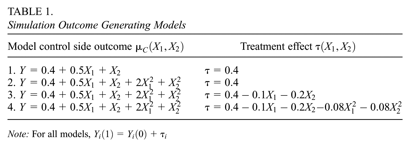
In addition to matching some of Porter et al.’s (2017) simulation parameters, we also explore parameter setups that are a closer match to empirical applications in education research. This involves using high running variable correlation parameters $ρ \in {0.95, 0.99}$ and a smaller sample size of $n = 1, 000$ in addition to Porter et al.’s (2017) sample size of $n = 5, 000$ . We show results using $n = 1, 000$ here and include results using $n = 5, 000$ , which were similar, in Supplemental Appendix Section 10.6.

Finally, the outcomes are generated as $Y_{i} = μ (X_{1 i}, X_{2 i}) + τ (X_{1 i}, X_{2 i}) W_{i} (X_{1 i}, X_{2 i}) + ϵ_{i}$ , with $μ (\cdot, \cdot)$ and $τ (\cdot, \cdot)$ under four different settings as shown in Table 1, following Porter et al. (2017) with residuals $ϵ_{i} ~^{iid} N (0, 1)$ . In models 1 and 2, the treatment effect is 0.4 everywhere along the boundary. In models 3 and 4, the treatment effect is heterogeneous along the boundary.

Table 1.

Simulation Outcome Generating Models

Model control side outcome $μ_{C} (X_{1}, X_{2})$	Treatment effect $τ (X_{1}, X_{2})$
1. $Y = 0.4 + 0.5 X_{1} + X_{2}$	$τ = 0.4$
2. $Y = 0.4 + 0.5 X_{1} + X_{2} + 2 X_{1}^{2} + X_{2}^{2}$	$τ = 0.4$
3. $Y = 0.4 + 0.5 X_{1} + X_{2} + 2 X_{1}^{2} + X_{2}^{2}$	$τ = 0.4 - 0.1 X_{1} - 0.2 X_{2}$
4. $Y = 0.4 + 0.5 X_{1} + X_{2} + 2 X_{1}^{2} + X_{2}^{2}$	$τ = 0.4 - 0.1 X_{1} - 0.2 X_{2}$ $- 0.08 X_{1}^{2} - 0.08 X_{2}^{2}$

Note: For all models, $Y_{i} (1) = Y_{i} (0) + τ_{i}$

Overall, we have four scenarios, two sample sizes, three cutoff pairs, and five running variable correlations, giving $4 \times 2 \times 3 \times 5 = 120$ simulation contexts. For each of these data generating models and parameter setups, we generate 500 simulated data sets. We apply each of the six methods to estimate the BATE and standard error for each simulated data set. A full list of parameters and BATE values for each data-generating model is listed in Supplemental Appendix Table 10.4. Our predictions, and correspondingly our treatment effect estimates, are scaled by the standard deviation of the control unit outcomes such that our results are in effect size units.

7.2. Implementation

We use the R package rddapp (Jin et al., 2021) to implement the binding score and pooled frontier methods (see Supplemental Appendix Section 10.1), specifying sharp two-dimensional RDDs. We also include the running variables as covariates in these models, which showed better precision in Porter et al. (2017). Gaussian process regression, loess, and the parametric surface response approaches are implemented as described in Sections 4, 5, and 6.

7.3. Results

We compare the performance of each method on its average absolute bias, precision, RMSE, coverage, and standard error estimation across data-generating models. We show results averaged over the three sets of running variable cutoff percentiles for the $n = 1, 000$ case as results are similar across the three choices. We do not see substantial gains in using precision-weighted Gaussian process regression and therefore show results here relative to density-weighted Gaussian process regression. Results showing precision-weighted Gaussian process regression, precision-weighted residualized Gaussian process regression, and precision-weighted loess are in Supplemental Appendix Section 10.5.

7.3.1. Comparison to Binding Score and Pooled Frontier

In Figure 2, the columns correspond to the numbered models in Table 1. The models in the first two columns have a constant treatment effect, while those in the third and fourth columns introduce heterogeneous treatment effects along the boundary. Additionally, models in columns two and four are more complex (they have curvature and interactions in the running variables) than the models in columns one and three. The rows of Figure 2 show our outcomes. In the first row, we compare the methods in terms of their absolute bias across simulations and simulation parameters. The second row shows their precision, and the third shows the RMSE.

Figure 2.

Simulation results averaged over running variable cutoff percentiles of 30/30, 50/50, and 30/70.

We first note that the differences between residualized and non-residualized Gaussian process regression’s outcomes are small in Figure 2. For example, in models 2 and 3, the bias difference between them is less than 0.001 effect size units for almost all running variable correlations, such that the non-residualized results are visually indistinguishable from the residualized Gaussian process regression results. In model 1, this bias difference is visible across running variable correlations but still small in effect size units. The middle and bottom rows of the figure show similar precision and RMSE, respectively, between residualized and non-residualized Gaussian process regression.

Overall, Gaussian process regression—both residualized and non-residualized—typically outperforms pooled frontier and binding score in terms of absolute bias, standard errors, and RMSE, especially as model complexity increases. The main exception is model 1, where the binding score shows comparable or slightly better performance at high running variable correlations; pooled frontier also performs well in model 1 at low correlations, but its bias worsens as correlation increases and in more complex models. In all other cases, Gaussian process regression consistently achieves lower bias, smaller standard errors, and lower RMSE than these alternatives.

Figure 3 shows the average coverage results of the BATE in the top panel using a 95% confidence interval. The bottom panel of this figure shows how well the methods estimated standard errors. All methods except the pooled frontier perform well for the simplest data setup, the first column. Across the other three data-generating models, Gaussian process regression continues to do well and outperforms binding score and pooled frontier in terms of both coverage and estimation of standard errors. Results are fairly similar between residualized and non-residualized density-weighted Gaussian process regression.

Figure 3.

Simulation coverage and standard error (SE) estimation across parameters.

7.3.2. Comparison to Surface Response Approaches

Given the limited differences between residualized and non-residualized Gaussian process regression in prior figures, we use only residualized Gaussian process regression in the remaining results. Figure 4 again shows results for the models in Table 1, this time for the parameter linear and quadratic approaches, the loess approach, and the Gaussian process regression approach. We see in this figure that, compared to loess regression and the parametric linear surface response approach, residualized Gaussian process regression does well in terms of absolute bias, precision, and RMSE. While loess consistently underperforms Gaussian process regression, the small differences between Gaussian process regression and the parametric linear surface response model in Model 1 grow dramatically in the more complex models. What Figure 4 also shows is that Gaussian process regression does not outperform the parametric quadratic surface response model, which is a correct specification of the data in models 2 to 4. This holds true for coverage and estimation of the true standard error as shown in Figure 5. However, the coverage of Gaussian process regression is otherwise relatively strong among surface response methods, with generally better coverage than a parametric linear surface response model, and more correct estimation of the true standard errors than loess regression.

Figure 4.

Simulation results averaged over running variable cutoff percentiles of 30/30, 50/50, and 30/70.

Figure 5.

Simulation coverage and standard error (SE) estimation across parameters.

In summary, residualized density-weighted Gaussian process regression performs better than the non-surface response methods across our data-generating models and simulated parameters. We find that it exhibits low bias and standard errors while maintaining good coverage and consistent recovery of the true standard errors. It also outperforms other nonparametric and parametric surface response methods, particularly when the parametric surface response approach is incorrectly specified. That said, Gaussian process regression does not, as expected, outperform a correctly-specified parametric surface response method. Taken together, Gaussian process regression exhibits the overall best performance of these methods in this simulation when the data-generating model is unknown.

8. Application: Wisconsin ELL Reclassification

To understand the methods’ comparative performance with real-world data, we use Gaussian process regression, binding score, pooled frontier, and loess to analyze an empirical two-dimensional RDD. We describe the data and policy context, define the estimand of interest, and show the results of analyzing the two-dimensional RDD using the different methods. We end with a demonstration of the capacity of Gaussian process regression to investigate heterogeneous treatment effects.

8.1. Policy Context

The two-dimensional RDD we use centers on the assignment of ELL students to non-ELL status based on their test scores in public high schools in Wisconsin. This change is known as reclassification, which indicates that these students are now considered to be fully English proficient. Reclassified students typically join mainstream classes with native English speakers and no longer receive English language instruction or linguistic accommodations.

In Wisconsin, ELL students in grades K–12 are tested annually in the winter on the ACCESS examinations, which measure English proficiency. ELL students receive ACCESS scores in multiple English language domains: Speaking, Listening, Reading, and Writing. Literacy is calculated as $Literacy = 50 % R e a d i n g + 50 % W r i t i n g$ . Students also receive an overall ACCESS score, which is a weighted average of the four domains: $Overall = 35 % Reading + 35 % W r i t i n g + 15 % L i s t e n i n g + 15 % S p e a k i n g$ (Wisconsin Depart-ment of Public Instruction, 2023). ACCESS scores are provided in terms of scale scores as well as proficiency levels, which range from 1.0 (lowest) to 6.0 (highest). Each proficiency level score corresponds to a cut point in the scale score. For example, a Literacy proficiency level of 5.0 requires a minimum scale score of 406 in the data we use.

From 2011 to 2016, Wisconsin state policy was to reclassify ELL students as non-ELL if they

(a) received a score of 6.0 on their Overall proficiency level score, or

(b) received a score of 5.0 on their Overall proficiency level score AND a score of at least 5.0 on their Literacy proficiency level score.

We examine the two-dimensional case of (b), where students were required to pass two thresholds to be eligible to receive the treatment of reclassification as a non-ELL. Even though there are technically two policy pathways to be labeled as a non-ELL, the rule of reclassification given at least a 5.0 on Literacy and a 5.0 on Overall fully determines who is reclassified and who is not, since anyone who scores a 6.0 on Overall also scores at least a 5.0 on Literacy. This means that we can conduct a two-dimensional RDD along the boundary defined by Literacy $\geq 5.0$ and Overall $\geq 5.0$ and employ the methods of this paper. Our research question is whether being eligible for mainstreaming into non-ELL classrooms helped students in terms of their academic outcomes, which in this case are their ACT test score results in the year after reclassification.

We examine the ELL reclassification policy for 10th-grade students. In Wisconsin, students typically take the ACT in the spring of 11th grade, meaning that the reclassification occurred one year prior to this outcome measure. Similar data were used by Carlson and Knowles (2016) to examine the impacts of reclassification for ELL students in Wisconsin on their ACT achievement, likelihood of high school graduation, and postsecondary enrollment following high school graduation, using the first rule (a) as the discontinuity in a fuzzy one-dimensional RDD. Using both linear and quadratic functional form specifications above and below the singular 6.0 cutoff on the Overall proficiency level score, Carlson and Knowles (2016) found that reclassification in 10th grade had a positive effect on students’ composite ACT scores, mainly driven by increases in English and Reading ACT scores.

Although reclassification under these policies in Wisconsin was intended to be automatic, there were students who passed these ACCESS test score thresholds but who were not classified as non-ELL students. This is partly due to the state’s manual reclassification policies, where automatically reclassified students could be manually classified back as ELL students if their districts deemed them not to be fully proficient in English. Manual reclassification was also possible in the other direction for students who scored a 5.0 on their Overall ACCESS score but less than a 5.0 on their Literacy ACCESS score, if the district determined that the students were in fact proficient in English. An additional explanation for discrepancies between passing ACCESS scores and reclassification status is that the automatic reclassification policy was a Wisconsin Department of Public Instruction recommendation without a strong forcing mechanism at the time. As such, there may have been delays between state-level automatic reclassification and district-level enacted reclassification of these students into non-ELL classrooms. Regardless, the counts of reclassified students were “relatively few” in either direction (Carlson & Knowles, 2016, p. 562).

These discrepancies motivate our examination of intent-to-treat effects of becoming eligible for reclassification after passing both score thresholds, as opposed to effects of reclassification itself, for this analysis. Furthermore, analyzing the two-dimensional nature of the policy allows us to assess potential treatment effect heterogeneity along the boundary. This gives us a more detailed perspective on which particular students are affected by ELL reclassification.

8.2. Data

Our analytic sample consists of all 10th-grade Wisconsin ELL students who were administered the ACCESS test between academic years 2010 to 2011 through 2015 to 2016 and who also took the ACT over that time, similarly to Carlson and Knowles (2016). This corresponds to 3,489 students.

In our data, 44% of students scored a 5.0 or above on Literacy, 52% scored a 5.0 or above on Overall, and 39% scored a 5.0 or above on both, meaning they passed the reclassification threshold. There were 2,038 students who did not meet the reclassification threshold in total. Of those students who did not pass, 3.9% scored a 5.0 or above on Literacy but not Overall (these students had Overall scores in the 4.0–4.9 range), and 17.1% scored a 5.0 or above on Overall, but not on Literacy.

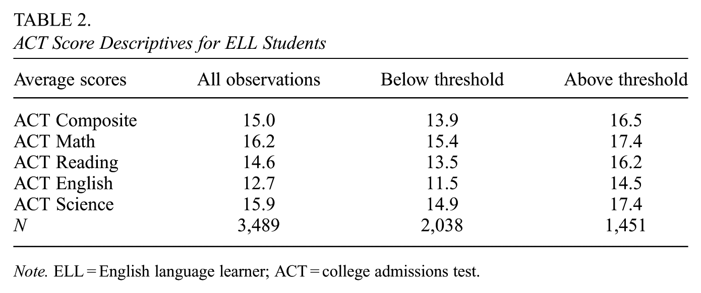
Table 2 presents statistics about these students’ ACT scores, which can range from 0 to 36. On average, ACT scores were higher for students whose ACCESS scores fell above the reclassification threshold than for students whose scores fell below. However, this difference is confounded by the fact that all students who were reclassified also performed better on the ACCESS test, which likely correlated with performance on the ACT test score. This motivates RDD methods, which aim to compare outcomes for students who barely were reclassified to those who barely were not.

Table 2.

ACT Score Descriptives for ELL Students

Average scores	All observations	Below threshold	Above threshold
ACT Composite	15.0	13.9	16.5
ACT Math	16.2	15.4	17.4
ACT Reading	14.6	13.5	16.2
ACT English	12.7	11.5	14.5
ACT Science	15.9	14.9	17.4
N	3,489	2,038	1,451

Note. ELL = English language learner; ACT = college admissions test.

The test score data are displayed in Figure 1 in Section 2, with student ACCESS Literacy scores along the x-axis and ACCESS Overall scores along the y-axis. The estimated correlation between the two running variables is high, 0.96, because a student’s Literacy score makes up part of their Overall score. Although the reclassification policy’s two passing rules are defined using ACCESS proficiency levels from 1.0 to 6.0, we use the proficiency levels’ corresponding scale scores to run our analysis, following Carlson and Knowles (2016), and we centered the running variables around their cutoffs. There is one scale score point that divides students who were eligible for treatment (the darker blue points in the top right of Figure 1) from those who were not eligible for treatment (the lighter blue points).

8.3. Estimand and Methods

We conduct inference on the $τ^{w}$ defined in Section 5 to estimate the BATE. This corresponds to estimating the average intent-to-treat effect of just barely passing the reclassification threshold boundary in 10th grade on ACT achievement. We examine results using both population density weights as well as precision weights. For outcomes, we consider all ACT skill area scores (English, Reading, Math, and Science) as well as students’ Composite ACT scores.

We compare the results of using Gaussian process regression, loess, binding score, pooled frontier, parametric linear surface response, and parametric quadratic surface response methods. We implemented these methods in the same way we had in the simulation study.

8.4. Results and Comparison

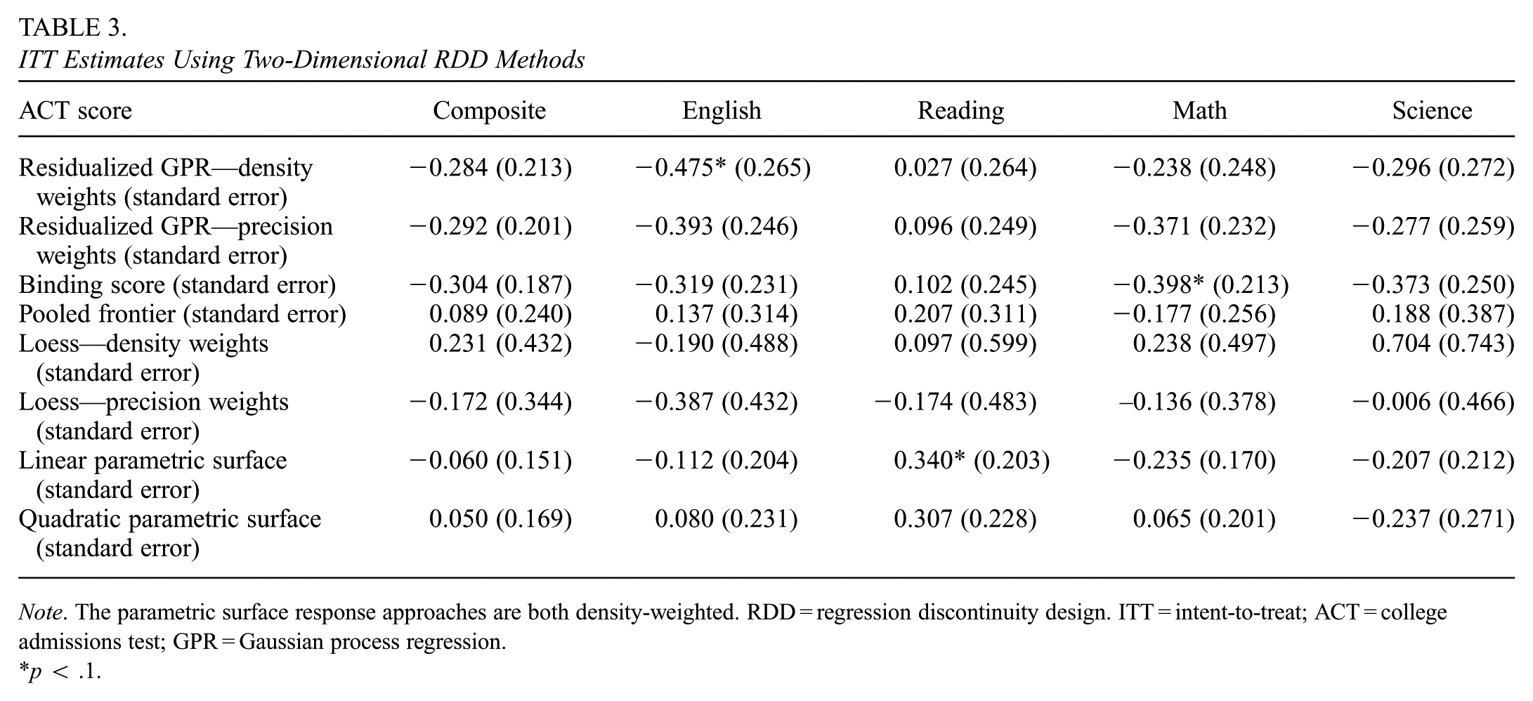
The results from all six methods are presented in Table 3. Each column represents one type of ACT test outcome estimate with standard errors in parentheses.³

Table 3.

ITT Estimates Using Two-Dimensional RDD Methods

ACT score	Composite	English	Reading	Math	Science
Residualized GPR—densityweights (standard error)	−0.284 (0.213)	−0.475* (0.265)	0.027 (0.264)	−0.238 (0.248)	−0.296 (0.272)
Residualized GPR—precision weights (standard error)	−0.292 (0.201)	−0.393 (0.246)	0.096 (0.249)	−0.371 (0.232)	−0.277 (0.259)
Binding score (standard error)	−0.304 (0.187)	−0.319 (0.231)	0.102 (0.245)	−0.398* (0.213)	−0.373 (0.250)
Pooled frontier (standard error)	0.089 (0.240)	0.137 (0.314)	0.207 (0.311)	−0.177 (0.256)	0.188 (0.387)
Loess—density weights(standard error)	0.231 (0.432)	−0.190 (0.488)	0.097 (0.599)	0.238 (0.497)	0.704 (0.743)
Loess—precision weights(standard error)	−0.172 (0.344)	−0.387 (0.432)	−0.174 (0.483)	−0.136 (0.378)	−0.006 (0.466)
Linear parametric surface(standard error)	−0.060 (0.151)	−0.112 (0.204)	0.340* (0.203)	−0.235 (0.170)	−0.207 (0.212)
Quadratic parametric surface (standard error)	0.050 (0.169)	0.080 (0.231)	0.307 (0.228)	0.065 (0.201)	−0.237 (0.271)

Note. The parametric surface response approaches are both density-weighted. RDD = regression discontinuity design. ITT = intent-to-treat; ACT = college admissions test; GPR = Gaussian process regression.

p < .1.

The only statistically significant results are for ACT English scores using residualized density-weighted Gaussian process regression, ACT Reading scores using a linear parametric surface response approach, and for ACT Math scores using binding score. These intent-to-treat effects are negative for ACT English and ACT Math, and positive for ACT Reading. Directionally, Gaussian process regression, binding score, precision-weighted loess, and linear parametric surface response results are almost all negative across ACT test results, excluding ACT Reading. Pooled frontier, density-weighted loess, and quadratic parametric surface response results are generally positive, though these are never significant.

When comparing the standard errors of the estimates across methods, precision-weighted Gaussian process regression estimates slightly outperform density-weighted. Meanwhile, pooled frontier and loess’s standard errors are larger than the Gaussian process regression results, while binding score and both parametric surface response results are slightly more precise. We conjecture that this performance is related to the 0.96 correlation between the running variables, and these results in terms of precision are in line with the lower standard errors for binding score results and higher standard errors for pooled frontier and loess that we saw in the simulation study under high running variable correlations (see Figure 2).

In Carlson and Knowles’s (2016) analysis of the fuzzy one-dimensional ELL reclassification RDD, they found estimated positive effects of reclassification that were 1 ACT Composite score point and 1.2 to 1.7 ACT English and Reading score points in magnitude. Though we similarly found a significant positive intent-to-treat effect of assignment to reclassification for ACT Reading using a linear parametric surface response approach, we, in contrast, found a significant but negative intent-to-treat effect for ACT English scores when analyzing the two-dimensional case using Gaussian process regression, though note that this effect is one-third the magnitude of Carlson and Knowles (2016). Though these two papers study the same state’s ELL reclassification policy, we analyzed the two-dimensional design while Carlson and Knowles (2016) focused on the one-dimensional version of the policy.

Importantly, using Gaussian process regression, we are able to visually investigate possible evidence of any heterogeneous treatment effects. Conducting this analysis allows us to understand if treatment has different effects for students with different patterns of test scores.

We use the ACT English test score outcome as an example here as it was found to be significant using Gaussian process regression. Figures for other ACT test outcomes are in Supplemental Appendix Section 10.8. In some cases, $\hat{BATEs}$ that are null overall can exhibit statistically significant effects at specific sentinels along the boundary, such as when sentinel-level results are both negative and positive and cancel out.

In Figure 6, the left panel shows the boundary defined by the 39 sentinels numbered from 1 to 39. Sentinel 20 is at the intersection of the two running variable cutoffs. The right panel shows the Gaussian process regression estimates (the light blue bars) using the ACT English score outcome. The accompanying orange whiskers represent pointwise 90% confidence intervals on each estimate. As expected given the distribution of data in the left panel, the standard error bars widen for sentinels further away from sentinel 20 as there is less data there. Note that the figure’s right hand panel only shows estimates for sentinels 12 to 25, meaning that sentinels 1 to 11 and 26 to 39 had too little data to estimate treatment effects and were therefore dropped, as explained in Section 5.3.

Figure 6.

Treatment effect heterogeneity along the boundary.

We provide the following interpretation of Figure 6 as an example of how one could use a figure like this, with sentinel-level estimates from Gaussian process regression, to investigate heterogeneous treatment effects along the boundary. Looking at the right-hand panel, we see that the magnitude and direction of the estimates vary over the sentinels, beginning with positive estimates for sentinels 12 to 15 and then showing negative estimates for the remaining sentinels. The confidence intervals show that the estimated treatment effects were significantly negative only for sentinels 18 through 20, and not significant otherwise. This provides evidence that the ELL reclassification policy functioned differently in terms of students’ English ACT scores for students who scored close to the ACCESS Literacy cutoff (those who just barely passed the Literacy cutoff, with an Overall score well above the cutoff along sentinels 12–15) or to the Overall cutoff with relatively high Literacy scores (along sentinels 21–25), compared to students who scored close to both cutoffs (along sentinels 18–20). Those students who scored closer to the intersection of the two running variable cutoffs experienced negative, statistically significant treatment effects of assignment to reclassification on their ACT English scores. This implies that the reclassification policy may be less helpful for students with this pattern of running variable scores that are both close to their cutoffs. In contrast, students who scored away from this intersection did not experience significant effects of assignment to reclassification. Interestingly, those students with both scores close to the cutoff were likely weaker students overall—suggesting they could have been reclassified too soon. A possible policy implication would be to change the cut scores of the reclassification policy.

9. Discussion

Two-dimensional RDDs—such as policies requiring students to meet thresholds on both English and mathematics exams to earn a high school diploma—are fairly common in educational research. However, most existing analytic methods reduce these two-dimensional RDDs to a single dimension. This simplification, while convenient for analysis, may be inappropriate when treatment effects vary along the full, multidimensional threshold.

In this article, we systematically compare traditional analytic techniques with both parametric and previously unexplored nonparametric surface response methods in educational settings. A central distinction between these approaches lies in how they treat the assignment boundary. The binding score and pooled frontier methods project the discontinuity to one-dimensional space to facilitate local linear regression, thereby losing valuable information. In contrast, surface response methods estimate treatment effects along the full two-dimensional threshold. This approach better captures the complexity of how interventions may impact individuals differently depending on where they cross into eligibility. Thus, it not only preserves the multidimensional structure of the data, but also facilitates the investigation of heterogeneous effects—essential for nuanced policy evaluation. The existence of policies involving three or more score-based cutoffs, such as the Math, ELA, and Science passing scores in Massachusetts’s high school Competency Determination requirement, further highlights the need for methodological approaches that fully model the data to capture the whole effect of the policy. Promising future work would be to develop surface response methods that allow for more than two running variables within an RDD. In theory, the Gaussian process regression approach presented here could be extended to this setting, with the caveat that investigating treatment effect heterogeneity and aggregating treatment effects to an overall measure would be more complex.

Flexibility in the surface response model is key. While not explored by Porter et al. (2017), parametric surface response models also allow the researcher to jointly model the treatment and control response surfaces and estimate the BATE as the difference. Unfortunately, such parametric methods can be difficult to use in practice given their sensitivity to the researcher’s choice of functional form (Porter et al., 2017). For example, in our comparison between a linear parametric surface response model and Gaussian process regression, when the true model is quadratic, the nonparametric approach had stronger performance. When correctly specified, parametric surface response models can be useful, but using nonparametric surface response methods reduces concerns regarding model misspecification.

Methodologically, our simulation design extends the frameworks of Porter et al. (2017) and Wong et al. (2013) by introducing highly correlated running variables and unknown, potentially nonlinear data-generating processes. We believe that this generates fairer comparisons between methods, as researchers typically cannot predict the existence of heterogeneous treatment effects or nonlinear data in advance.

Across a range of settings, including those closely mirroring Porter et al. (2017), Gaussian process regression exhibited robust performance across all running variable correlations, data-generating processes, and running variable cutoffs. Though Porter et al. (2017) found the frontier and binding score methods to have good statistical properties, our simulations reveal that the pooled frontier method is generally either more biased or less precise than Gaussian process regression. Gaussian process regression also demonstrated much better coverage and estimation of standard errors than the other methods, with the binding score method exhibiting lower coverage under more complex data-generating models. For the least complex data setups, the binding score showed similarly strong properties to Gaussian process regression and would be simpler to implement using conventional RDD methods. However, researchers may not be able to reliably assess the complexity of their data, and so we recommend using Gaussian process regression, which showed strong performance regardless of data complexity.

Gaussian process regression also performed well in comparison to the other surface response approaches. Despite also being a nonparametric surface response method, loess regression tended to exhibit higher bias and standard errors, as well as worse estimation of the true standard errors than Gaussian process regression. On the parametric side, the parametric linear surface response approach showed poor performance when the model was truly quadratic, showing that it was vulnerable to model misspecification. Collectively, these results indicate that, among all methods considered, Gaussian process regression may be the safest approach in scenarios with an unknown data-generating model.

The above said, actual running variable distributions may be bounded or skewed. In all these simulations, the two running variables are drawn from Normal distributions with varying correlations. While this approach extends to empirical running variables that are fairly Normal, bounded or skewed running variables may present analytical challenges that future research should examine. This may be more concerning when the skew affects one running variable but not the other—in this case, the running variables would have quite different distributions. Wong et al. (2013) found that under those circumstances, using raw versus standardized running variables affected BATE estimates.

Our simulations focus on the ability of surface response methods to estimate the BATE, but this may not be their greatest advantage. Both the density-weighted and precision-weighted overall BATE estimates can be difficult to conceptualize, especially when there is a large degree of impact heterogeneity. This is especially true for the precision-weighted estimate, which is targeting an estimand defined simply by its ease of estimation. Regardless, any single number representing a weighted average of a mixture of people as described by different values of the pair of running variables, with different responses to treatment, can be overly simplistic if there is notable impact variation, and should, in such cases, be accompanied by a description of the heterogeneity of the estimated curve. If there is little evidence of heterogeneity, however, then the single number can be taken as a more general representation of the impact (for those along the boundary), and the weighting choice is less important as well.

This is where the Gaussian process approach adds value: beyond its statistical advantages for BATE estimation, Gaussian process regression allows for visual, intuitive inspection of potential treatment effect heterogeneity for individuals with different patterns of running variables. In our case, for example, our results suggest that overall null BATE estimates may mask a mix of positive and negative effects for students at different points along the treatment boundary. By recognizing the differences in both running variables and outcomes of students at different points along the boundary, future policymakers could, potentially, direct programs differentially to students and therefore target students who may benefit the most. Thus, overall we recommend that researchers and policymakers use tools such as Gaussian process regression to try to understand not only the average effect, however defined, but also to characterize treatment effect heterogeneity.

We close with some advice for applied researchers on using these tools:

First, researchers have several decisions in implementing Gaussian process regression, but, fortunately, many of these decisions do not overly matter. We show in the Supplemental Appendix that the number of sentinels, dropping low-weight sentinels, and the use of precision-weighted versus density-weighted estimates have little effect on the GP estimation. Between anisotropic and isotropic kernels, we recommend using an anisotropic kernel, especially if the running variables measure different constructs. We recommend using a precision weights-based BATE as these will generally correspond with the more interpretable density weights when units are fairly regularly distributed, and they also mitigate concerns with scaling of the running variables. That said, density weights are more interpretable, especially when the running variables are on similar scales.

Generally, we advocate using Gaussian processes. That said, if one thought treatment were generally constant along the entire boundary in a case with running variables on the same metric, then the binding score method would be a reasonable choice. The frontier methods can also be useful if the target of interest were the BATE for each boundary segment. The binding score method is limited, however, if the running variables measure different constructs.

Finally, we note again that summarizing a two-dimensional RDD as one $BATE$ estimate may be unduly reductive, especially if the treatment curve $τ (x)$ varies substantially. In these cases, researchers should at a minimum report both treatment effects along each boundary or, even better, provide the fully estimated curve, in addition to using the BATE to succinctly describe the policy’s effect.

To ease the technical challenges of implementing these methods and generating these tools, we provide an R package, twodrdd. This package also contains a vignette that demonstrates estimation and visualization.

Supplemental Material

sj-pdf-1-jeb-10.3102_10769986251403088 – Supplemental material for Improving Estimation for Two-Dimensional Regression Discontinuity Designs in Education With Gaussian Process Regression

Supplemental material, sj-pdf-1-jeb-10.3102_10769986251403088 for Improving Estimation for Two-Dimensional Regression Discontinuity Designs in Education With Gaussian Process Regression by Lily An, Zach Branson and Luke W. Miratrix in Journal of Educational and Behavioral Statistics

Footnotes

Declaration of Conflicting Interests

The authors declared no potential conflicts of interest with respect to the research, authorship, and/or publication of this article.

Funding

The authors disclosed receipt of the following financial support for the research, authorship, and/or publication of this article: This work was supported by Grant R305B150010 to Harvard University from the Institute of Education Sciences, U.S. Department of Education.

ORCID iDs

Lily An

Luke W. Miratrix

Notes

Authors

LILY AN is an assistant professor in the Department of Educational Policy Studies at Georgia State University, 30 Pryor Street SW, Atlanta, GA, 30303; e-mail: lan2@gsu.edu. Her research interests are in educational policy analysis, measurement, and school accountability.

ZACH BRANSON is an associate teaching professor in the Department of Statistics and Data Science at Carnegie Mellon University, 5000 Forbes Avenue, Pittsburgh, PA 15213; e-mail: zach@stat.cmu.edu. His research interests are experimental design and causal inference.

LUKE W. MIRATRIX is a professor of education in the Harvard Graduate School of Education at Harvard University, Massachusetts Hall, Cambridge, MA 02138; e-mail: luke_miratrix@gse.harvard.edu. His research interests are in causal inference and treatment effect heterogeneity.

References

Alcantara

Wang

Hahn

P. R.

Lopes

(2024). Modified BART for learning heterogeneous effects in regression discontinuity designs. arXiv Preprint, 2024, arXiv:2407.14365.

Athey

Imbens

G. W.

(2017). The state of applied econometrics: Causality and policy evaluation. Journal of Economic Perspectives, 31(2), 3–32.

Branson

Mealli

(2018). Local randomization and beyond for regression discontinuity designs. arXiv Preprint, 2018, arXiv:1810.02761.

Branson

Rischard

Bornn

Miratrix

L. W.

(2019). A nonparametric Bayesian methodology for regression discontinuity designs. Journal of Statistical Planning and Inference, 202(2), 3.

Calonico

Cattaneo

M. D.

Farrell

M. H.

(2018). On the effect of bias estimation on coverage accuracy in nonparametric inferenc. Journal of the American Statistical Association, 113(522), 767–779.

Calonico

Cattaneo

M. D.

Titiunik

(2014). Robust nonparametric confidence intervals for regression-discontinuity designs. Econometrica, 82(6), 2295–2326.

Carlson

Knowles

(2016). The effect of English language learner reclassification on student ACT scores, high school graduation, and postsecondary enrollment: regression discontinuity evidence from Wisconsin. Journal of Policy Analysis and Management, 35(3), 559–586.

Cattaneo

M. D.

Frandsen

B. R.

Titiunik

(2015). Randomization inference in the regression discontinuity design: An application to party advantages in the US Senate. Journal of Causal Inference, 3(1), 1–24.

Cattaneo

M. D.

Titiunik

(2022). Regression discontinuity designs. Annual Review of Economics, 14, 821–851.

10.

Cattaneo

M. D.

Titiunik

Vazquez-Bare

(2017). Comparing inference approaches for RD designs: A reexamination of the effect of Head Start on child mortality. Journal of Policy Analysis and Management, 36(3), 643–681.

11.

Chib

Greenberg

Simoni

(2023). Nonparametric bayes analysis of the sharp and fuzzy regression discontinuity designs. Econometric Theory, 39(3), 481–533.

12.

Chib

Jacobi

(2016). Bayesian fuzzy regression discontinuity analysis and returns to compulsory schooling. Journal of Applied Econometrics, 31(6), 1026–1047.

13.

Cleveland

W. S.

Devlin

S. J.

(1986). Locally weighted regression: An approach to regression analysis by local fitting. Journal of the American Statistical Association, 83, 596–610.

14.

Cohodes

S. R.

Goodman

J. S.

(2012). First degree earns: The impact of college quality on college completion rates. HKS Faculty Research Working Paper Series.

15.

Dee

(2012). School turnarounds: Evidence from the 2009 stimulus (Technical report). National Bureau of Economic Research.

16.

Díaz

J. D.

Zubizarreta

J. R.

(2023). Complex discontinuity designs using covariates: Impact of school grade retention on later life outcomes in Chile. The Annals of Applied Statistics, 17(1), 67–88.

17.

Geneletti

O’Keeffe

A. G.

Sharples

L. D.

Richardson

Baio

(2015). Bayesian regression discontinuity designs: incorporating clinical knowledge in the causal analysis of primary care data. Statistics in Medicine, 34(15), 2334–2352.

18.

Gramacy

R. B.

(2016). LaGP: Large-scale spatial modeling via local approximate Gaussian processes in R. Journal of Statistical Software, 72(1), 1–46. https://doi.org/https://doi.org/10.18637/jss.v072.i01

19.

Hahn

Todd

Van der Klaauw

(2001). Identification and estimation of treatment effects with a regression-discontinuity design. Econometrica, 69(1), 201–209.

20.

Hahn

P. R.

Murray

J. S.

Carvalho

(2020). Bayesian regression tree models for causal inference: regularization, confounding, and heterogeneous effects. Bayesian Analysis, 15(3): BA1195.

21.

Imbens

Lemieux

(2008). Regression discontinuity designs: A guide to practice. Journal of Econometrics, 142(2), 615–635.

22.

Imbens

Zajonc

(2011). Regression discontinuity design with multiple forcing variables (Report, Harvard University).

23.

Jacoby

W. G.

(2000). Loess: A nonparametric, graphical tool for depicting relationships between variables. Electoral Studies, 19(4), 577–613.

24.

Jin

Liao

Papst

Zhang

Hochstedler

Thoemmers

(2021). rddapp: Regression Discontinuity Design Application [R package version 1.3].

25.

Kane

T. J.

(2003). A quasi-experimental estimate of the impact of financial aid on college-going (Technical report). National Bureau of Economic Research.

26.

Keele

Titiunik

Zubizarreta

J. R.

(2015). Enhancing a geographic regression discontinuity design through matching to estimate the effect of ballot initiatives on voter turnout. Journal of the Royal Statistical Society: Series A (Statistics in Society), 178(1), 223–239.

27.

Keele

L. J.

Titiunik

(2015). Geographic boundaries as regression discontinuities. Political Analysis, 23(1), 127–155.

28.

Mattei

Mealli

(2015). Evaluating the causal effect of university grants on student dropout: evidence from a regression discontinuity design using principal stratification. The Annals of Applied Statistics, 9(4), 1906–1931.

29.

Ludwig

Miller

D. L.

(2007). Does Head Start improve children’s life chances? Evidence from a regression discontinuity design. The Quarterly Journal of Economics, 122(1), 159–208.

30.

Martorell

(2005). Do high school graduation exams matter? A regression discontinuity approach [Unpublished manuscript. University of California Berkeley, 28].

31.

(2010). To leave or not to leave? A regression discontinuity analysis of the impact of failing the high school exit exam. Economics of Education Review, 29(2), 171–186.

32.

Papay

J. P.

Murnane

R. J.

Willett

J. B.

(2010). The consequences of high school exit examinations for low-performing urban students: Evidence from Massachusetts. Educational Evaluation and Policy Analysis, 32(1), 5–23.

33.

Papay

J. P.

Murnane

R. J.

Willett

J. B.

(2014). High-school exit examinations and the schooling decisions of teenagers: Evidence from regression-discontinuity approaches. Journal of Research on Educational Effectiveness, 7(1), 1–27.

34.

Papay

J. P.

Willett

J. B.

Murnane

R. J.

(2011). Extending the regression-discontinuity approach to multiple assignment variables. Journal of Econometrics, 161(2), 203–207.

35.

Pei

Lee

D. S.

Card

Weber

(2022). Local polynomial order in regression discontinuity designs. Journal of Business & Economic Statistics, 40(3), 1259–1267.

36.

Porter

K. E.

Reardon

S. F.

Unlu

Bloom

H. S.

Cimpian

J. R.

(2017). Estimating causal effects of education interventions using a two-rating regression discontinuity design: Lessons from a simulation study and an application. Journal of Research on Educational Effectiveness, 10(1), 138–167.

37.

Rasmussen

C. E.

Williams

C. K. I.

(2006). Gaussian processes for machine learning. MIT Press.

38.

Reardon

S. F.

Arshan

Atteberry

Kurlaender

(2010). Effects of failing a high school exit exam on course taking, achievement, persistence, and graduation. Educational Evaluation and Policy Analysis, 32(4), 498–520.

39.

Reardon

S. F.

Robinson

J. P.

(2012). Regression discontinuity designs with multiple rating-score variables. Journal of Research on Educational Effectiveness, 5(1), 83–104.

40.

Rischard

Branson

Miratrix

Bornn

(2021). A Bayesian nonparametric approach to geographic regression discontinuity designs: Do school districts affect NYC house prices? Journal of the American Statistical Association, 116(534), 619–631.

41.

Robinson

J. P.

(2011). Evaluating criteria for English learner reclassification: A causal-effects approach using a binding-score regression discontinuity design with instrumental variables. Educational Evaluation and Policy Analysis, 33(3), 267–292.

42.

Sekhon

J. S.

Titiunik

(2017). On interpreting the regression discontinuity design as a local experiment. In Regression discontinuity designs: Theory and applications (pp. 1–28). Emerald Publishing Limited.

43.

Stein

M. L.

(1999). Interpolation of spatial data: Some theory for kriging. Springer.

44.

Thistlethwaite

D. L.

Campbell

D. T.

(1960). Regression-discontinuity analysis: An alternative to the ex post facto experiment. Journal of Educational Psychology, 51(6), 309.

45.

Wisconsin Department of Public Instruction. (2023). WISEdash for Districts ACCESS Dashboards. https://dpi.wi.gov/wisedash/districts/about-data/access

46.

Wong

V. C.

Steiner

P. M.

Cook

T. D.

(2013). Analyzing regression-discontinuity designs with multiple assignment variables: A comparative study of four estimation methods. Journal of Educational and Behavioral Statistics, 38(2), 107–141.

Supplementary Material

Please find the following supplemental material available below.

For Open Access articles published under a Creative Commons License, all supplemental material carries the same license as the article it is associated with.

For non-Open Access articles published, all supplemental material carries a non-exclusive license, and permission requests for re-use of supplemental material or any part of supplemental material shall be sent directly to the copyright owner as specified in the copyright notice associated with the article.

0.00 MB

0.73 MB