A Partial Linear Estimator for Small Study Regression Discontinuity Designs

Abstract

Regression discontinuity (RD) designs are a popular approach to estimating a treatment effect of cutoff-based interventions. Two current estimation approaches dominate the literature. One fits separate regressions on either side of the cutoff, and the other performs finite sample inference based on a local randomization assumption. Recent developments of these approaches have often focused on asymptotic properties and large sample sizes. Educational applications often contain relatively small samples or sparsity near the cutoff, making estimation more difficult. As an alternative to the aforementioned approaches, we develop a partial linear estimator for RD designs. We show in simulations that our estimator outperforms certain leading estimators in several realistic, small-sample scenarios. We apply our estimator to school accountability scores in Indiana.

Keywords

regression discontinuity nonparametric semiparametric partial linear small sample

1. Introduction

Regression discontinuity (RD) designs are a quasi-experimental framework originally developed by Thistlethwaite and Campbell (1960). In the classic RD design, a treatment is assigned to all individuals who score above a certain cutoff of a continuous running variable, and linear regression is used to estimate the causal effect of the treatment. The prevalence of cutoff-based interventions in the fields of economics and education has made RD designs a popular causal inference method in recent decades and has led to important methodological advances.

Currently, two approaches dominate the RD literature. The first, popularized by Hahn et al. (2001), relies on assumptions about the continuity of the underlying mean function. Practitioners typically fit separate models on either side of the cutoff and estimate the average treatment effect (ATE) as the difference between the values of the response predicted at the cutoff based on the two models. Nonparametric regression is often preferred due to the local nature of RD designs (Gelman & Imbens, 2019), necessitating that users choose a tuning parameter called a bandwidth. Popular algorithms calculate bandwidths optimized for different inferential methods, including those proposed by Armstrong and Kolesár (2020; henceforth AK), Calonico et al. (2014; henceforth CCT), and Imbens and Kalyanaraman (2012; henceforth IK).

The second approach to RD estimation was popularized by Cattaneo et al. (2015), who rely on local randomization (LR), that is, the idea that observations near the cutoff fall on either side of the cutoff essentially at random. Practitioners typically choose a window near the cutoff where the LR is assumed to hold and then use finite sample methods to estimate the ATE. Much like for bandwidths in the continuity approach, much of the current research in this area focuses on algorithms to automatically choose the window.

Much recent methodological development has focused on economic applications, where the sample sizes are typically quite large. Swartzentruber and Kaizar (2024), henceforth SK, note that educational applications often feature smaller sample sizes or samples that are sparse around the cutoff. SK compare the performance of popular RD estimation methods within both major approaches. Simulation results show that some methods known to have desirable asymptotic qualities do not work particularly well with small or sparse samples. These methods require extra estimation in order to achieve those asymptotic gains, and without enough data to effectively perform that extra estimation their small-sample performance suffers.

In this article, we propose a method that outperforms currently popular RD estimation methods in many small sample scenarios. Our method is an implementation of the partial linear RD estimator explored by Porter (2003), henceforth Porter. The partial linear approach has been neglected in the literature, perhaps because Porter shows some asymptotic inferiorities compared to the approach that fits separate models on either side of the cutoff. We argue that these asymptotic results are not relevant for small or sparse samples, for which the partial linear approach has certain desirable qualities. We develop a tailored bandwidth selection algorithm and variance estimation technique and use simulation to show that our partial linear estimator tends to have better operating characteristics than competing methods in several realistic small sample scenarios.

The article is organized as follows: Section 2 describes the local polynomial estimation method that dominates the continuity approach and contrasts it with Porter’s original partial linear estimator. Section 3 highlights the modifications we make to Porter’s estimator, including the details of our bandwidth selection algorithm and variance estimation technique. In Section 4, we present the results of a simulation study comparing our method to several competing methods. We provide a real-data example using school accountability scores in Section 5 before concluding in Section 6.

2. Overview of Select RD Estimation Methods

In this article, we focus on the sharp RD design, in which treatment D is based solely on the relationship between the value of the continuous running variable X and the cutoff c, namely $D = 1_{[X \geq c]}$ . Let Y be a continuous response variable. We define the true underlying mean function as $E (Y | X) = μ (x) = μ^{-} (x) 1_{[X < c]} + μ^{+} (x) 1_{[X \geq c]}$ , where $μ^{-} (x)$ and $μ^{+} (x)$ are the mean functions below and above the cutoff, respectively. We are interested in estimating the ATE at the cutoff, $τ = μ^{+} (c) - μ^{-} (c)$ .

Hahn et al. (2001) advocate for the use of local polynomial regression to separately estimate $μ^{-} (x)$ and $μ^{+} (x)$ and use these to estimate $τ$ . This nonparametric method employs a user-supplied kernel function, bandwidth, and polynomial degree to estimate the mean at a given point as a weighted average of the response values close to that point. Here, we will refer to this method as local polynomial estimation (LPE). Local constant regression (LPE with polynomial degree 0) is known to suffer from bias when estimating near boundary points, and thus, Hahn et al. (2001) advocate the use of local linear regression as a way to mitigate this bias.

As an alternative to LPE, Porter considers an approach based on partial linear models, which are semiparametric models with both a parametric and a nonparametric component. Porter recognizes that an RD model can be written as

Y_{i} = τ D_{i} + μ^{*} (X_{i}) + ϵ_{i},

(1)

where $μ^{*} (X_{i}) = μ (X_{i}) - τ D_{i}$ is the underlying nonparametric mean function with the discontinuity $τ$ subtracted from points above the cutoff. Porter rewrites the model as $Y_{i} - τ D_{i} = μ^{*} (X_{i}) + ϵ_{i}$ , allowing $Y - τ D$ to become the response variable. He then writes out an expression for the least squares criteria and estimates $τ$ by minimizing that objective function:

\hat{τ} = \underset{τ}{\arg \min} \sum_{i = 1}^{n} {[y_{i} - τ d_{i} - \sum_{j = 1}^{n} l_{j} (x_{i}) (y_{j} - τ d_{j})]}^{2} .

(2)

where l_j are the weights used in the nonparametric regression calculated via a kernel function and bandwidth.

This estimator is equivalent to one proposed for general partial linear models by Robinson (1988), who shows that Equation 1 implies that $Y_{i} - E (Y | X_{i}) = τ (D_{i} - E (D | X_{i})) + ϵ_{i}$ . He uses the residuals from two constant regression estimations, $Y_{i} - \hat{E} (Y | X_{i})$ and $D_{i} - \hat{E} (D | X_{i})$ to estimate $τ$ by applying a no-intercept OLS model and proved the consistency of the resulting estimator. Porter shows that different consistency properties arise if D is a deterministic function of X, as for the RD model, but the conceptualization of Robinson (1988) motivates the variance estimation technique we develop in Section 3.

One important distinction between this semiparametric estimator and the currently popular two-model estimator is that, for partially linear estimator (PLE), the behavior of $μ^{*} (X)$ at the cutoff x=c should follow any constraints, such as “smoothness,” imposed by the mean function estimator chosen by the practitioner. Thus, PLE estimators use data from both sides of the cutoff to estimate the underlying mean function. One potential advantage of using a single nonparametric mean function is that this estimator is not vulnerable to the same boundary bias as the estimator that uses two separate local polynomial regression models. Exploring this feature of PLE, Porter derives asymptotic distributions of $\hat{τ}$ based on local constant regression under two sets of smoothness assumptions for the underlying mean function and uses asymptotic variance to develop plug-in standard error formulas. The weaker assumption requires continuity in $μ^{*} (X_{i})$ at the cutoff with finite derivatives on either side, while the stronger assumption requires these derivatives to be equal.

Porter compares the asymptotic properties of the LPE and his PLE. He shows that when the stronger smoothness assumption holds, both the PLE and the LPE achieve optimal rates of convergence, but the PLE does not in general achieve the optimal rate when only the weaker smoothness assumption holds. The LPE is able to achieve the optimal rate under the weaker assumption, although the degree of the local polynomial needed depends on the amount of smoothness. He concludes by advocating for the use of the LPE based on potential robustness, a point reiterated by Van Der Klaauw (2008). Perhaps due to this recommendation, the PLE has been given scant attention in the literature over the last 20 years.

3. Implementation of the Partial Linear Estimator

While the partial linear model may not be asymptotically superior, the PLE’s reliance on smoothness at the cutoff and use of data on both sides of the cutoff may reduce the variability of the treatment effect estimate and thus mitigate the limited statistical power due to sparse data near the cutoff. However, unlike for LPE where a rich array of nonparametric models have been explored, to our knowledge the local constant regression is the only nonparametric model that has been fully examined and implemented for use with PLE for RD analyses. In this article, we fill this gap in the literature by proposing broader options for the weights, along with a customized bandwidth algorithm and method for approximating the standard error.

Porter shows that using weights based on local constant regression with PLE does not suffer from the poor boundary properties that would come from using such weights in the two-model approach. While Porter suggested the use of higher-order kernels for further bias reduction in certain situations, he did not pursue this avenue to full implementation. Marron (1994) notes that asymptotic gains from the use of higher-order kernels in nonparametric regression often require quite large sample sizes and that there are other drawbacks such as the poor interpretability of negative weights. For these reasons, and to be more in line with the rest of the RD estimation literature, we also do not pursue higher-order kernels here. Rather, motivated by the relationship between higher-order kernels and higher-order local polynomial regression (see Fan et al., 1997; Yu, 2016), we modify Porter’s estimator in Equation 2 to use local polynomial weights $l = l^{LP}$ of a general degree p, and denote the resulting effect size estimator ${\hat{τ}}^{PLE}$ .

The solution to the minimization is easily seen in matrix form. Let Y be the $n \times 1$ vector of responses. Let $l^{(i)} = {(l_{1}^{L P} (x_{i}), \dots, l_{n}^{L P} (x_{i}))}^{'}$ be the vector of weights for x_i, and let these vectors be combined into the n×n weight matrix $L = (l^{(1)}, \dots, l^{(n)})$ . Let $D = (1_{{x_{1} \geq c}}, \dots, 1_{{x_{n} \geq c}})$ be a $n \times 1$ vector of treatment indicators. Finally, let $G = (I - L^{T}) D$ . Then, it can be shown that

{\hat{τ}}^{P L E} = {(G^{'} G)}^{- 1} G^{'} (I - L^{'}) Y,

(3)

which is a linear combination of the observed responses.

In addition to the polynomial degree, the weights depend on the choice of kernel and bandwidth. Following the advice from Fan and Gijbels (1996), LPE methods often employ the triangular kernel because it is thought to be optimal for boundary estimation. But since the cutoff is no longer at a boundary in the PLE method, we focus on the use of the optimal interior estimation Epanechnikov kernel to calculate the local polynomial weights.

3.1. PLE Bandwidth Selection Algorithm

Porter does not provide a bandwidth selection algorithm optimized for PLE with local constant weights. He suggests that cross-validation could be used, but this is no longer a common RD bandwidth selection approach, and it would be difficult to apply in a small sample setting. One could certainly pair other popular bandwidth selection algorithms with PLE. However the popular bandwidth algorithms from IK and CCT rely on the assumption that the second derivatives of $μ^{*} (X)$ differ at the cutoff. But recall that the motivation for the PLE involves estimating a single smooth mean function $μ^{*} (X)$ , from which the discontinuity is subtracted from points receiving the treatment. Thus, we make use of the stronger of Porter’s two smoothness assumptions:

Assumption 1. Right and left-hand derivatives of $μ^{*} (X)$ to order $λ_{μ}$ are equal at c.

We expect that in many educational applications we will not see substantial deviations from this smoothness assumption. Noteworthy large-sample RD educational studies, such as Abdulkadiroğlu et al. (2014), Lindo et al. (2010), and Martorell and McFarlin (2011), present data in which the smoothness assumption seems reasonable. Assumption 1 also seems reasonable for the data in our empirical application, which we discuss in Section 5. Furthermore, our simulation study in Section 4 shows that the PLE approach can still perform well in small sample regimes with modest deviations from Assumption 1.

Porter proves the following result about $\hat{τ}$ with local constant functions and second-order kernels, which are equivalent to ${\hat{τ}}^{PLE}$ with p= 0.

Theorem 1. If Assumption 1 holds with $λ_{μ} \geq 3$ and $h^{3} \sqrt{nh} \to A$ , where $0 \leq A < \infty$ , then

\sqrt{nh} (\hat{τ} - τ) \to^{d} N (A b_{P}, C_{P 1} \frac{σ_{+}^{2} (c) + σ_{-}^{2} (c)}{4 f (c)}),

(3)

where ${b_{P} = 2 K_{2} (0) {(f (c) \int_{0}^{\infty} K_{0}^{2} (w) d w)}^{- 1} (\frac{f^{'} (c)}{f (c)} g_{2} (c) \int_{0}^{\infty} K_{1} (v) d v - g_{2}^{'} (c) \int_{0}^{\infty} K_{0} (v) v d v)$ ,

g_{2} (x) = μ^{*^{'}} (x) f^{'} (x) + μ^{*} (x) f (x) / 2,

(3)

and K₀, K₁, K₂, and C_P1 are functions of the chosen kernel.

From this distribution, we derive the asymptotic mean squared error (MSE) of $\hat{τ}$ with local constant regression to be

{AMSE}_{PLE} (h) = h^{6} b_{P}^{2} + \frac{C_{P 1} (σ_{+}^{2} (c) + σ_{-}^{2} (c))}{4 nhf (c)} .

(4)

By minimizing this expression with respect to the bandwidth h we arrive at an infeasible optimal bandwidth, which we denote h_SM in reference to the smoothness assumption on which it relies:

h_{SM} = \underset{h}{\arg \min} AMS E_{PLE} (h) = {(\frac{C_{P 1} (σ_{+}^{2} (c) + σ_{-}^{2} (c))}{24 {nb}_{P}^{2} f (c)})}^{1 / 7} .

(5)

For a fully data-driven plug-in bandwidth ${\hat{h}}_{SM}$ , we must estimate the unknown quantities in the expression above. For this estimation, we often modify ideas from the plug-in approaches of IK, CCT, and Arai and Ichimura (2018), which require the estimation of similar quantities. The plug-in estimands fall into three main categories: the density of the running variable and its derivatives, the derivatives of the underlying mean function, and the variance function. We address each category in turn.

3.1.1. Estimating the Density of the Running Variable and Its Derivatives

The expression for b_P involves the density of the running variable and its first and second derivatives evaluated at the cutoff. As discussed in Jones (1994), kernel density estimation and kernel density derivative estimation are fairly standard ways to estimate the density of an unknown function and its derivatives, respectively.

For some bandwidth h and kernel K, we can estimate the density f(x) with

\hat{f} (x) = \frac{1}{n} \sum_{i = 1}^{n} \frac{1}{h} K (\frac{x - X_{i}}{h}) .

(6)

To calculate derivatives of the density at a point, we choose to follow the seemingly most popular and widely implemented approach, which is to simply differentiate the right hand side of Equation 6. This approach requires the kernel to be piece-wise differentiable on its support and the derivative to be nonconstant on that support. To meet these requirments, we employ the Gaussian kernel, $K (x) = \frac{1}{\sqrt{2 π}} e^{- \frac{1}{2} x^{2}}$ , rather than the Epanechnikov or triangular kernels often used in RD estimation. For consistency we use this kernel for the density estimation as well. We implement this estimation using the kdde function in the ks package (Duong, 2022) in R. We use the well-known plug-in estimator of Wand and Jones (1994) to choose the bandwidth.

3.1.2. Estimating Derivatives of the Mean Function

To estimate b_P we also need estimates of the first three derivatives of the underlying mean function. This is perhaps the most challenging of the quantities needed, especially considering that our ultimate goal involves estimating the underlying mean function itself. IK, CCT, and Arai and Ichimura (2018) propose slightly different multistage approaches that make use of local polynomial techniques. We incorporate some of their ideas in our estimation, but one important distinction is that since we are assuming the derivatives of the mean function are the same on both sides of the cutoff, we need one overall estimate for each derivative rather than one on each side.

We take as our starting point the infeasible optimal bandwidth formula for estimating the $ν$ th derivative of a function at a point in the interior of the function’s support from Fan and Gijbels (1996),

h_{FG} = C_{FG} (ν, ρ, K) {(\frac{σ^{2} (c)}{{(μ^{*^{(ρ + 1)}})}^{2} f (c) n})}^{1 / (2 ρ + 3)},

(7)

where $ρ$ is the degree of the local polynomial we are using to approximate the underlying mean function, and $C_{FG} (ν, ρ, K)$ is a constant that depends on $ν$ , $ρ$ , and the kernel K. Since this formula is for an interior point, we use the optimal Epanechnikov kernel in the calculation of this constant. This formula is optimal when $ρ - ν$ is odd. We choose to use $ρ = ν + 1$ for $ν \in {1, 2, 3}$ .

For each value of $ρ$ , we need an estimate of the derivative $μ^{*^{(ρ + 1)}}$ . We achieve this in a similar manner to IK, by fitting global polynomials that include a treatment indicator. Fan and Gijbels (1996) suggest fitting a polynomial of degree $ρ + 3$ , but we feel that such a high degree would not be ideal in a small sample scenario. Instead, we follow the strategy of CCT and fit polynomials of degree $ρ + 1$ . Thus, we fit global polynomials with a jump at the cutoff of degree 3, 4, and 5 (corresponding to $ρ =$ 2, 3, and 4, respectively), and from these polynomials, we calculate $μ^{* (ρ + 1)}$ for each $ρ$ .

Equation 7 also requires a plug-in estimate of the variance function at the cutoff, $σ^{2} (c)$ . We mirror the approach of Arai and Ichimura (2018) to use the estimated variance from the polynomial regression, which assumes homoscedasticity, rather than the estimate of the variance function in Section 3.1.3. However, for f(c), we do use the same value estimated in Section 3.1.1. Plugging in these quantities gives data-driven pilot bandwidths ${\hat{h}}_{FG}$ for each of $ν \in {1, 2, 3}$ .

IK, CCT, and Arai and Ichimura (2018) all use their pilot bandwidths in subsequent local polynomial regressions on either side of the cutoff as described above. However, we are unable to use traditional LPE at this stage because we are estimating a single mean function with a structurally imposed discontinuity. Rather, we incorporate ideas from both parametric and nonparametric methods. We restrict our data to just those observations within one bandwidth of the cutoff, essentially using a uniform kernel similar to the approach of IK. However, rather than fitting a regular polynomial like IK does, we fit a polynomial with a treatment indicator on this subset of our data similar to the polynomial we fit globally in the first stage of our approach. We choose the degree of the polynomial we fit at this stage to be equal to the value of $ρ$ . From these polynomials, we calculate the desired derivatives $μ^{*^{(ν)}} (c)$ . for $ν \in {1, 2, 3}$ .

3.1.3. Estimating the Variance Function

The numerator of h_SM involves $σ_{+}^{2} (c)$ . and $σ_{-}^{2} (c)$ , the right- and left-hand limits of the variance function at the cutoff. Note that we are not assuming here a constant variance function and thus desire separate calculations using data on either side of the cutoff. Arai and Ichimura (2018) use variance estimates obtained from their estimation of the mean function derivatives described in Section 3.1.2. However, we assumed homoscedasticity that stage and do not want to plug in that single variance estimate for both values.

We use a nearest-neighbor approach similar to CCT in the hope that it will lead to more stable estimates for small samples. Thus, we estimate the variance below and above the cutoff as

{\hat{σ}}_{-}^{2} (c) = \frac{1}{J - 1} \sum_{i = 1}^{J} {(Y_{i, -} - {\bar{Y}}_{-})}^{2}

(8)

and

{\hat{σ}}_{+}^{2} (c) = \frac{1}{J - 1} \sum_{i = 1}^{J} {(Y_{i, +} - {\bar{Y}}_{+})}^{2},

(9)

where J is the number of nearest neighbors, $Y_{i, -}$ and $Y_{i, +}$ are the response values for the J unique observations with X_i values closest to the cutoff, below and above the cutoff, respectively, and ${\bar{Y}}_{-}$ and ${\bar{Y}}_{+}$ are the average of the J response values below and above the cutoff, respectively. For our implementation, we follow CCT to choose J=3.

3.2. PLE Variance Estimation

To conduct inference in the RD setting using our PLE estimator, we must choose a variance estimation technique. Porter proposes variance estimation based on the asymptotic distribution of the PLE estimator. However, for small studies this asymptotic distribution may be quite different from the true distribution of $\hat{τ}$ . We advocate for using an approach based on jackknife resampling. In Supplemental Appendix Section A2, we present alternative approaches based on jackknife resampling as well as a direct plug-in approach and show via simulation that our favored jackknife approach performs relatively well.

The jackknife is a resampling procedure that typically removes one observation at a time from a dataset, calculates an estimate based on the remaining n−1 observations, and then utilizes those n point estimates to estimate the variance of the overall estimate. You and Chen (2003) estimate the variance by applying a jackknife formula from Hinkley (1977) designed for a linear model to the parametric second step of the general partial linear estimation technique of Robinson (1988). This approach involves deleting one pair of residuals $(Y_{i} - \hat{E} (Y | X_{i}), D_{i} - \hat{E} (D | X_{i}))$ each time, rather than one original observation, in order to estimate the parametric coefficient $τ$ . We modify their method, using a jackknife formula that Wu (1986) shows to have the same double robustness property as that of Hinkley (1977) but is also unbiased in the case of homogenous error variances. The result is our PLE variance estimator,

{\hat{V}}_{P L E} ({\hat{τ}}^{P L E}) = \sum_{i = 1}^{n} (1 - w_{i}) {({\hat{τ}}_{(i)}^{P L E} - {\hat{τ}}^{P L E})}^{2} = {({\hat{D}}^{'} \hat{D})}^{- 2} \sum_{i = 1}^{n} \frac{r_{i}^{2}}{1 - w_{i}} {\hat{d}}_{i}^{2},

(10)

where ${\hat{d}}_{i} = d_{i} - \hat{E} (d | x_{i})$ , $\hat{D} = {({\hat{d}}_{1}, ... {\hat{d}}_{n})}^{'}$ , $r_{i} = y_{i} - \hat{E} (y | x_{i}) - {\hat{d}}_{i} \hat{τ}$ , $w_{i} = {\hat{d}}_{i}^{'} {({\hat{D}}^{'} \hat{D})}^{- 1} {\hat{d}}_{i}$ , and ${\hat{τ}}_{(i)}^{PLE}$ is the treatment effect estimate with the i th pair of residuals removed.

This choice of variance estimation allows us to approximate a PLE $(1 - α) 100 %$ confidence interval as

I_{PLE} = {\hat{τ}}^{PLE} \pm z_{α / 2} {SE}^{PLE} (\hat{τ}),

(11)

where ${SE}^{PLE} (\hat{τ}) = \sqrt{{\hat{V}}_{PLE}}$ .

4. Simulation Study

In this section, we present the results from a Monte Carlo simulation study comparing the operating characteristics of PLE methods developed in Section 3 to several leading RD estimation methods.

We first consider the conventional continuity method in which a point estimate is calculated by fitting separate local linear regressions with a triangular kernel on either side of the cutoff where the bandwidth is selected via the MSE-optimal bandwidth algorithm designed for it by IK. We refer to this method as CV/IK.

Our second comparator method is the robust, bias-corrected (RBC) approach of CCT. They estimate and correct for the bias of the conventional point estimate as well as inflate the standard error estimate to account for the added variability that comes from this bias correction. Their bandwidth algorithm utilizes the same asymptotic formulas as IK but differs in the estimation of the mean and variance functions required for a data-driven result. We refer to this method as RBC/CCT.

Our third comparator method is based on the idea of fixed-length confidence intervals (FLCI) of AK. They use the conventional point estimate, but inflate the critical value in order to achieve better confidence interval coverage. They also develop a bandwidth algorithm that pairs with their inferential technique. Their formulas rely on the second derivative bound of the underlying mean function, but they also propose a data-driven approximation of this value, which we use in our simulation. We refer to this method as FLCI/AK.

We also consider the LR methods of Cattaneo et al. (2015), which rely on finite sample inference in a window close to the cutoff. They propose a window selection method that is not feasible for the simulation that we are performing here. Thus, we follow the approach of SK and choose a window based on guaranteeing a minimum number of observations within that window. We use 5, 10, and 20 for this minimum, and refer to these methods as LR/LR5, LR/LR10, and LR/LR20, respectively. This ad-hoc window selection may not perform as well as data-driven methods often used in practice, and there are differences in the assumptions and causal estimands between the continuity and LR frameworks, so we must be cautious in such comparisons.

In addition to these existing methods, we consider methods based on the PLE inferential approach given by Equations 3 and 11. This requires a choice of degree p for the local polynomial weights. The bandwidth developed in Section 3.1 is optimal for p= 0, but using p= 1 is more in line with the continuity methods considered above. Thus, we consider both specifications paired with the SM bandwidth (Equation 5) and refer to these as PLE0/SM (p= 0) and PLE1/SM (p= 1). We recognize that the SM bandwidth is not technically optimal for p= 1 but will show that it still works fairly well in practice. We leave the development of an optimal bandwidth for p= 1 to future work. In addition to the SM bandwidth, we also pair both PLE specifications with the IK bandwidth, which we will show works well with the PLE approach despite the conflicting assumptions mentioned earlier. We refer to these methods as PLE0/IK and PLE1/IK. In all PLE methods, we use the Epanechnikov kernel.

We use R (v4.4.0; R Core Team, 2024) for all calculations. We use the package rdrobust (v2.2; Calonico et al., 2023) for the CV/IK and RBC/CCT methods, the package RDHonest (v1.0.0; Kolesár, 2024 and v0.3.2; Kolesár, 2021) for the FLCI/AK method, the package rdlocrand (v1.0; Cattaneo et al., 2022) for the LR methods, and the package rdple (v1.0.0; Swartzentruber, 2025) for the PLE methods.

4.1. Simulation Study Settings

We consider four data generating processes (DGPs) that differ in the distribution of the running variable as well as the underlying mean function $μ$ , and are illustrated in Figure 1. To generate values of the running variable X_i, we first draw independent values Z_i from a particular Beta distribution, and then transform them using $X_{i} = 2 Z_{i} - 1$ so that the support of the running variable is $[- 1, 1]$ . The cutoff is set to be c= 0. The response values Y_i are generated from the values of the running variable X_i as $Y_{i} = μ (X_{i}) + ϵ_{i}$ , where $ϵ_{i} ~^{iid} N (0, {. 1295}^{2})$ . This is similar to the approaches taken in the simulation studies of CCT, IK, and SK.

Figure 1.

Mean function $μ (x)$ (solid line) and density $f (x)$ (dashed line) of the DGPs.

The first three DGPs are taken from the SK simulation. DGP1 is a modified version of a DGP from the simulation of AK. It has a flat Beta(1,1) distribution for Z and a mean function consisting of quadratic splines with nodes not at the cutoff. DGP2 comes from the simulation of IK and is based on data from Lee (2008). The variable Z has a Beta(2,4) distribution, which means that approximately 19% of the density is above the cutoff. The mean function consists of quintic polynomials on either side of the cutoff that differ only in their intercept. DGP3 is modeled after the Indiana school accountability data from SK that we also analyze in Section 5. It has a Beta(14,7) distribution for Z with less than 6% of its density below the cutoff, and a mean function consisting of separate cubic polynomials on either side of the cutoff. DGP4 uses a Beta(1,1) distribution for Z, but its underlying mean function is flat on either side of the cutoff, meeting the assumption of the LR method. The equations of the mean functions are

\begin{matrix} μ_{DGP 1} (x) = {(x + 1)}^{2} - 2 s (x + 0.2) + 2 s (x - 0.2) - 2 s (x - 0.4) + 2 s (x - 0.7) - 0.92 \\ + (0.1) 1_{[x \geq 0]} \end{matrix}

(12)

μ_{DGP 2} (x) = 0.42 + 0.84 x - 3.0 x^{2} + 7.99 x^{3} - 9.01 x^{4} + 3.56 x^{5} + (0.1) 1_{[x \geq 0]}

(13)

\begin{matrix} μ_{DGP 3} (x) = (0.05 + 1.5 x + 3.2 x^{2} + 2.7 x^{3}) 1_{[x < 0]} \\ + (0.15 - 0.15 x + 2.5 x^{2} - 1.5 x^{3}) 1_{[x \geq 0]} \end{matrix}

(14)

μ_{DGP 4} (x) = (0.1) 1_{[x \geq 0]}

(15)

where $s (x) = {(x)}_{+}^{2} = \max {x, 0}^{2}$ is the square of the plus function. Each mean function has a discontinuity of 0.1. Note that $μ_{DGP 1}$ , $μ_{DGP 2}$ , and $μ_{DGP 4}$ all satisfy Assumption 1, so we might expect the PLE estimators to perform well in these simulations, whereas for $μ_{DGP 3}$ they may be inferior to the comparators that do not require smoothness at the cutoff.

Sample size and sparsity both contribute to the amount of information available for estimation at the cutoff. We consider different distributions of running variables because we are interested in the performance of RD estimation methods when there are varying levels of sparsity near the cutoff. However, this makes it difficult to determine the samples sizes to use in such a simulation. For example, a sample of size 500 with a Beta(1,1) distribution yields approximately 250 values on either side of the cutoff, while that same sample size with a Beta(14,7) distribution yields only about 30 observations below the cutoff and 470 above the cutoff. The amount of information available near the cutoff is quite different for these scenarios.

Thus, for setting up our simulation, we employ the density inclusive study size (DISS) metric $\bar{m}$ developed by SK, which is the expected number of observations within a Silverman rule of thumb bandwidth of the cutoff for a given sample size and running variable distribution. Because this bandwidth is calculated based solely on the distribution of the running variable and is thus agnostic to the bandwidth algorithm or inferential method employed in the RD estimation, we do not expect to systematically advantage one method over another by selecting sample size based on method-specific tailored algorithms. SK demonstrate this advantage, as well as how the DISS metric promotes the ability to compare results across simulation settings with different running variable distributions. Table 1 gives the sample sizes for the values of $\bar{m}$ that we consider in our simulation study, identical to those in SK. We generate 50,000 simulated datasets for each combination of $\bar{m}$ and DGP.

Table 1.

Sample Sizes for the Different DGPs at Each Value of $\bar{m}$ , Which Have Been Rounded to the Nearest Whole Number

DGP	$\bar{m} = 10$	$\bar{m} = 21$	$\bar{m} = 27$	$\bar{m} = 44$	$\bar{m} = 57$
DGP1/DGP4	40	101	140	256	354
DGP2	56	140	194	354	490
DGP3	140	354	494	905	1,254

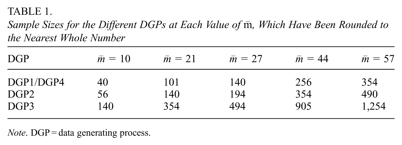
Note. DGP = data generating process.

4.2. Simulation Study Results

We evaluate the RD estimation methods in terms of both point and interval estimation. One complication in doing so is the differing rates at which the estimation and interval calculation algorithms successfully produce finite numeric results with default settings. At the larger study sizes, there is near universal success. However, at the smaller study sizes, some of the simulated datasets are so sparse near the cutoff that some of the methods are unable to obtain finite estimates. For the sake of a fair comparison, the summaries presented in this section are calculated from the simulated data sets in which all methods obtained finite estimates for a particular DGP and study size. For $\bar{m} = 10$ , this represents between 48.06% and 82.56% of all simulated datasets. For $\bar{m} = 21$ , this represents at least 98.49% of simulated datasets. For the larger study sizes, this represents at least 99.86% of all simulated datasets. Due to the difficulty of estimation for $\bar{m} = 10$ , as well as to simplify the graphical displays, we focus on study sizes of 21, 27, and 44 in this section but report estimates for all study sizes in the Supplemental Appendix.

Another potential complication in interpreting the results of our simulation study is that because our methods employ different bandwidth algorithms, they naturally have a different effective sample sizes. Figure 2 shows the average bandwidth value for each of the different algorithms considered. The AK algorithm consistently produces the smallest bandwidths, followed by CCT. The IK algorithm tends to produce the largest bandwidths, although SM has larger average values for DGP4. Certainly differences in point and interval estimation we see in our results are related to bandwidth size. However, our goal here is to compare our novel approach to other popular estimators, and differences in effective sample size are part of that comparison. In unreported simulations, we look at the other combinations of bandwidth algorithms and inferential techniques, for example, PLE1/CCT. We find that the PLE approach tends to outperform the comparator methods when using their own bandwidth algorithm, but does not perform as well as when using the IK or SM algorithm, and thus we do not present those results here.

Figure 2.

Average bandwidth values for the continuity methods for the four DGPs at three of our study sizes $(\bar{m})$ .

For point estimation we consider the following metrics: $bias = \frac{1}{n} \sum_{i = 1}^{n} (\hat{τ_{i}} - τ)$ , empirical standard error (EmpSE) $= \sqrt{\frac{1}{n - 1} \sum_{i = 1}^{n} {(\hat{τ_{i}} - \bar{τ})}^{2}}$ , and MSE $= \sqrt{\frac{1}{n} \sum_{i = 1}^{n} {(\hat{τ} - τ)}^{2}}$ . For easier graphical comparison we also use the square root of the MSE (RMSE). For interval estimation, we consider the median width of the intervals produced as well as the nominal coverage of those intervals.

4.2.1. Point Estimation

Figure 3 depicts the RMSE values for the continuity methods for the four DGPs at three of our study sizes ( $\bar{m}$ ). See Supplemental Appendix Table A1 for MSE values at the other two study sizes.

Figure 3.

RMSE for continuity methods at three study sizes. Observations not shown have RMSE values more than 0.15. Exact MSE values and Monte Carlo standard errors are given in Supplemental Appendix Table A1.

We begin by comparing the PLE methods. For DGP3 and DGP4, there is little difference between PLE0 and PLE1 for either considered bandwidth algorithm. PLE1 performs better in DGP1, while PLE0 performs better in DGP2, although in the latter case, there is less of a difference between the methods. We gain further insight into these relationships by considering the two components of the RMSE, the bias and the EmpSE, whose values are displayed for the same scenarios in Figure 4 and Supplemental Appendix Tables A2 and A3. The PLE1 methods have a much higher bias than PLE0 for DGP2. Recall from Figure 1 that the curvature varies considerably below the cutoff for DGP2 and thus for small sample sizes, a local linear approach may be more susceptible to overestimating the treatment effect than a local constant approach. In the other DGPs, the curvature varies less and PLE1 has bias values at or below PLE0 as we might expect.

Figure 4.

Absolute value of the bias and EmpSE for continuity methods at three study sizes. Observations not shown have EmpSE values more than 0.23. Exact values and Monte Carlo standard errors are given in Supplemental Appendix Tables A2 and A3.

We also note that the PLE methods often work better with the IK bandwidth rather than with the supposedly optimal SM bandwidth. PLE1/IK has lower RMSE values than PLE1/SM for three of the four DGPs and is competitive in the fourth. PLE0/IK has lower RMSE values than PLE0/SM for two of the four DGPs and is competitive in the other two. PLE1/IK is perhaps the top performing method overall in these scenarios. It has the lowest RMSE value for all considered sample sizes for both DGP1 and DGP3 and is competitive for the other DGPs.

Overall, the PLE methods perform well relative to the comparator methods in terms of point estimation. In particular, the PLE methods tend to have much smaller EmpSE than the RBC/CCT and FLCI/AK methods, although these comparator methods do tend to outperform the PLE methods in terms of bias. One possible factor in these comparisons is that the CCT and AK algorithms produce smaller bandwidths, on average, than the IK and SM algorithms. However, in unreported simulations, the RBC method did not perform markedly better when paired with the IK algorithm. Combining the bias and EmpSE into the RMSE, we see that both the RBC/CCT and FLCI/AK methods are never among the competitive methods and are in fact dominated by all the PLE methods in nearly all reported scenarios. The only comparator method that is sometimes competitive in terms of RMSE is CV/IK. However, this method is bested by either PLE0/IK or PLE1/IK in all DGPs at all study sizes in our simulation.

Supplemental Appendix Figure A1 compares the bias, EmpSE, and RMSE values for the PLE and LR methods. As expected, the LR methods perform quite well in terms of RMSE in DGP4, in which the LR assumption holds, particularly when using the LR20 window. If the underlying mean function is truly flat, then using more observations will lead to better results. However, for larger study sizes, the PLE methods are competitive with the LR methods in this DGP. For the DGPs that do not satisfy the LR assumption, the PLE methods generally outperform the LR methods in terms of RMSE, particularly for more serious violations of this assumption. In DGP2, for example, the underlying mean function is relatively flat near the cutoff but has rapidly increasing curvature below the cutoff. For larger study sizes or windows, the LR methods are able to avoid using points in the more curved area and perform well, although for each considered study size one of the PLE methods still has the minimum RMSE. DGP1, on the other hand, has a more serious violation of the LR assumption near the cutoff, leading to high bias and noncompetitive RMSE for the LR methods.

4.2.2. Interval Estimation

We evaluate interval estimation in terms of the empirical coverage of the nominally 95% confidence intervals produced by the different methods as well as the median width of the intervals, which are plotted for the continuity methods in Figure 5 for the middle study size of $\bar{m} = 27$ . Supplemental Appendix Figures A2 and A3 display the same metrics at the other study sizes, and Supplemental Appendix Tables A4 and A5 give exact values of these metrics and Monte Carlo standard errors for all study size and methods, including the LR methods that are not shown in the figures. Ideally, we would like to see correct coverage produced by small intervals so the best methods will have a summary near the dark line and further left in each panel of the figures.

Figure 5.

Median interval widths and empirical coverage for nominally 95% confidence intervals for all methods at study size $\bar{m} = 27$ . The graph omits the observation for PLE0/IK for DGP3, which has coverage of 0.81 and a median interval width of 0.17. Exact values and Monte Carlo standard errors are given in Supplemental Appendix Tables A4 and A5.

The PLE0 and PLE1 methods tend to have similarly small median interval widths within each DGP. However, they sometimes exhibit lower than nominal coverage, particularly in cases where the point estimation is biased. The PLE1 methods outperform PLE0 in coverage in DGP1 and DGP3, where they are also less biased, while the opposite is true in DGP2. The differences between the PLE methods using the SM and IK bandwidths are fairly modest in most scenarios, although PLE1/IK is perhaps still the top overall performer.

The FLCI/AK method tends to exhibit the best coverage of all considered methods for most scenarios, although it is edged out by one or both of the PLE1 methods for larger DGP3 study sizes. However, this comes at the cost of very wide intervals. The RBC/CCT method also produces fairly wide intervals, but is typically not competitive in terms of coverage. As in point estimation, CV/IK is the comparator method most similar to that of the PLE methods, with relatively narrow intervals and modest coverage. The LR methods again do very well in DGP4 but elsewhere exhibit low coverage due in large part to biased point estimates.

4.2.3. Summary of Results

Considering both point and interval estimation, the PLE methods tend to outperform the comparator methods in our simulation settings. Overall, the top performer in our simulation is the PLE1/IK method. For DGP1 and DGP3, it outperforms both continuity and LR methods. For DGP2, PLE1/IK outperforms the LR methods and is competitive with the continuity methods. Each of these represents a realistic scenario for an applied researcher, with DGP2 and DGP3 based on real data sets. DGP4 is a more contrived scenario that in many ways represents the best case for LR methods. PLE1/IK is competitive there as well, although a more sophisticated window algorithm that could take advantage of more of the data may have given a much larger edge to the LR methods.

There are three perhaps somewhat surprising takeaways regarding our novel methods. The first is that on the whole, PLE1/SM tends to outperform PLE0/SM in our settings, despite the SM algorithm being optimal for local constant regression. In certain scenarios PLE0/SM works quite well, but in other scenarios, it is noncompetitive, whereas PLE1/SM is much more competitive in the scenarios when it is not optimal. Recall that the PLE estimator is not subject to the poor boundary properties that cause Hahn et al. (2001) to recommend local linear regression. Despite this, these results may indicate that there are other benefits of using PLE1 instead PLEO in small sample cases. However, without further exploration and more extensive simulations, we do not have a definitive answer on the optimality of PLE1 versus PLE0.

The second takeaway is that PLE inference tends to work as well or better with the IK bandwidth algorithm than with SM, which is unexpected given the contradictory assumptions mentioned in Section 3.1. This may be an indication that the unknown quantities in Equation 5 are more difficult to estimate with small samples than those in the corresponding IK infeasible bandwidth. A potentially more substantial issue, however, is that in our SM algorithm we are still using an asymptotic expression as a starting point for a method designed for finite sample inference. Thus, we see the SM bandwidth algorithm as a preliminary result, and we hope it can be improved upon in the future. However, the performance of PLE with both IK and SM also shows that the PLE method is somewhat robust to choice of bandwidth selection algorithm.

The final takeaway is that the link between Assumption 1 and PLE performance is not as strong as we would have thought. The PLE estimators perform well in DGP3, despite a violation to the smoothness assumption. The strengths of the PLE approach appear to outweigh the magnitude of the assumption violation in this particular example. However, had the violation been more severe, we may have seen a different result. Certainly more work is needed, perhaps in the form of future simulation studies, to explore the impact of smoothness on PLE estimation.

5. Data Application

An example of educational data with sparsity near the cutoff of a running variable is the Indiana school accountability score data set first analyzed by SK. In this section, we use our partial linear estimator to estimate the effect of the threat of sanctions on failing Indiana schools. However, the goal of this analysis is the demonstration of our methods, and we do not perform any of the RD assumption checks and sensitivity analyses that would be necessary to make a rigorous policy recommendation.

Beginning with the 2015 to 2016 school year, the Indiana Department of Education (2022) implemented a new accountability system in which each school was given a numeric score between 0 and 120. Schools that scored below a 60 were considered to be failing schools. The system outlined sanctions for schools that received failing grades multiple years in a row. The sanctions varied depending on the type of school and the number of consecutive failing years. We have data on these school accountability scores from the years 2017 and 2018, the first 2 years of full publicly available data (Indiana Department of Education, 2017, 2018). A scatterplot of the data is given in Figure 6.

Figure 6.

A scatterplot of the Indiana school accountability data. The dashed line represents the cutoff. The solid line represents the estimated mean function using the PLE/SM method, and the vertical part of that line at the cutoff represents the PLE/SM treatment effect estimate.

This dataset can be analyzed as a sharp RD design. The running variable is a school’s score in the year 2017, and the response variable is the score in the year 2018. Since none of the sanctions take place after only 1 year of receiving a failing grade, the treatment is the threat of sanctions rather than the sanctions themselves. Presumably, the Indiana Department of Education would like the threat of sanctions to motivate failing schools to improve their scores in the following year. If that is true, than the scores should be higher slightly below the cutoff than they are slightly above. This would lead to a negative value of $τ$ by the definition given earlier.

Out of the 1933 schools in the dataset, 88 were given a failing score in 2017, representing less than 5% of the total. This is an example of a sparse data situation where the vast majority of the density of the running variable is far from the cutoff. There are m= 51 values within a rule of thumb bandwidth of the cutoff and thus by the DISS metric falls between the $\bar{m} = 44$ and $\bar{m} = 57$ settings from our simulation, despite a larger overall sample size.

From Figure 6, we can also see that Assumption 1, which requires equal derivatives of the mean function on either side of the cutoff, seems reasonable. This makes some intuitive sense. Most of the students and teachers at these schools in 2018 were also there in 2017 and making substantial change in education is typically not a short-term process. Failing schools may certainly see differences in factors such as morale, motivation, and community support compared to passing schools that may impact their 2018 scores, but the consistent composition of the schools means that in both groups we would expect a school with a slightly higher score than another school in 2017 to have a similar slightly higher score than the other in 2018.

Using our PLE1/SM method, we estimate the ATE to be 2.44, meaning that the threat of sanctions causes a decrease of 2.44 points in the following year’s accountability score. This point estimate can be seen in Figure 6, along with the estimated mean function. This estimated treatment effect is indeed in the opposite direction of what the Department of Education would presumably like. A 90% confidence interval for this effect is [−2.97, 7.85], so we do not have statistically discernible evidence of an effect in either direction. If the Department of Education was hoping to increase school accountability scores by the threat of sanctions, it does not appear that their goal was met. However, we reiterate that this is a preliminary analysis that is limited in real-world interpretability.

Figure 7 gives point estimates and confidence intervals for this treatment effect from the other methods considered in our simulation study. The differences between methods here mirrors that of the simulation study. The PLE methods and the CV/IK methods give relatively narrow intervals with similar centers, although the PLE0 methods produce a relatively larger treatment effect estimate. The FLCI/AK interval is more than twice as wide as the PLE intervals, fully containing them, and the RBC/CCT interval is also relatively wide. It would appear that the LR assumption might not be reasonable in a very large window, leading to potential bias for the LR methods. This is particularly true when using the LR10 window, which results in a confidence interval completely above zero.

Figure 7.

Point estimates and 90% confidence intervals for the treatment effect for various methods.

6. Conclusion

RD designs are an important tool for applied researchers estimating causal effects of cutoff-based interventions in a variety of fields. Many of the methods that have been developed in recent years focus on asymptotic or large-sample properties, which likely led to researchers discounting the potential of the asymptotically inferior PLE approach. However, there are many applications with relatively small sample sizes or sparsity near the cutoff. There is a need for RD estimation methods that cater to these situations. Because PLE simultaneously incorporates points on both sides of the cutoff to estimate a single smooth mean function, PLE is a good candidate for small sample RD estimation.

We introduced a new partial linear estimator that modifies Porter’s original method to include local polynomial weights. We developed an MSE-optimal bandwidth algorithm that leverages an underlying smoothness assumption that is realistic in many RD settings. We paired our estimator with a jackknife-based variance estimation technique for inference. We showed that the resulting PLE methods are always competitive with and often outperform certain popular methods in a set of small sample data scenarios. In our simulations, the top performing method was our PLE1 approach paired with the IK bandwidth selection algorithm.

The methods we developed have a strong potential to help researchers working with small sample RD designs. We further hope that our work sparks renewed interest in small study RD estimation methods. In the future, we plan to refine our current bandwidth algorithm to improve its performance, develop a new bandwidth algorithm that is optimal for the local linear PLE1, and to extend our methodology to fuzzy RD designs and other, more complicated, design structures.

Supplemental Material

sj-pdf-1-jeb-10.3102_10769986261417636 – Supplemental material for A Partial Linear Estimator for Small Study Regression Discontinuity Designs

Supplemental material, sj-pdf-1-jeb-10.3102_10769986261417636 for A Partial Linear Estimator for Small Study Regression Discontinuity Designs by Daryl Swartzentruber and Eloise Kaizar in Journal of Educational and Behavioral Statistics

Footnotes

Declaration of Conflicting Interests

The authors declared no potential conflicts of interest with respect to the research, authorship, and/or publication of this article.

Funding

The authors received no financial support for the research, authorship, and/or publication of this article.

ORCID iD

Daryl Swartzentruber

Authors

DARYL SWARTZENTRUBER is an assistant professor of Data Science and Mathematics at Centre College, 600 West Walnut Street, Danville, KY 40422; email: daryl.swartzentruber@centre.edu. His research interests are regression discontinuity designs and other types of causal inference, particularly for educational and sports analytics applications.

ELOISE KAIZAR is a professor of Statistics and the Chair of the Statistics Department at The Ohio State University, 1958 Neil Ave, Columbus, OH 43210; email: kaizar.1@osu.edu. Her research interests include causal inference and population-relevant inference.

References

Abdulkadiroğlu

Angrist

Pathak

(2014). The elite illusion: Achievement effects at Boston and New York exam schools. Econometrica, 82(1), 137–196. https://doi.org/10.3982/ECTA10266

Arai

Ichimura

(2018). Simultaneous selection of optimal bandwidths for the sharp regression discontinuity estimator. Quantitative Economics, 9(1): 441–482. https://doi.org/10.3982/QE590

Armstrong

T. B.

Kolesár

(2020). Simple and honest confidence intervals in nonparametric regression. Quantitative Economics, 11(1), 1–39. https://doi.org/10.3982/QE1199

Calonico

Cattaneo

M. D.

Farrell

M. H.

Titiunik

(2023). rdrobust: Robust Data-Driven Statistical Inference in Regression-Discontinuity Designs. Comprehensive R Archive Network (CRAN), R package version 2.2. https://CRAN.R-project.org/package=rdrobust

Calonico

Cattaneo

M. D.

Titiunik

(2014). Robust nonparametric confidence intervals for regression-discontinuity designs. Econometrica, 82(6), 2295–2326. https://doi.org/10.3982/ECTA11757

Cattaneo

M. D.

Frandsen

B. R.

Titiunik

(2015). Randomization inference in the regression discontinuity design: An application to party advantages in the U.S. senate. Journal of Causal Inference, 3(1), 1–24. https://doi.org/10.1515/jci-2013-0010

Cattaneo

M. D.

Titiunik

Vazquez-Bare

(2022). rdlocrand: Local Randomization Methods for RD Designs. Comprehensive R Archive Network (CRAN), R package version 1.0. https://CRAN.R-project.org/package=rdlocrand

Duong

(2022). ks: Kernel Smoothing. Comprehensive R Archive Network (CRAN), R package version 1.13.5. https://CRAN.R-project.org/package=ks

Fan

Gasser

Gijbels

Brockmann

Engel

(1997). Local polynomial regression: Optimal kernels and asymptotic minimax efficiency. Annals of the Institute of Statistical Mathematics, 49(1), 79–99. https://doi.org/10.1023/A:1003162622169

10.

Fan

Gijbels

(1996). Local polynomial modelling and its applications. Chapman and Hall.

11.

Gelman

Imbens

(2019). Why high-order polynomials should not be used in regression discontinuity designs. Journal of Business & Economic Statistics, 37(3), 447–456. https://doi.org/10.1080/07350015.2017.1366909

12.

Hahn

Todd

Van der Klaauw

(2001). Identification and estimation of treatment effects with a regression-discontinuity design. Econometrica, 69(1), 201–209. https://doi.org/10.1111/1468-0262.00183

13.

Hinkley

D. V.

(1977). Jackknifing in unbalanced situations. Technometrics, 19(3), 285–292. https://doi.org/10.1080/00401706.1977.10489550

14.

Imbens

Kalyanaraman

(2012). Optimal bandwidth choice for the regression discontinuity estimator. The Review of Economic Studies, 79(3), 933–959. https://doi.org/10.1093/restud/rdr043

15.

Indiana Department of Education. (2017). 2017 A-F school grade reports [Data file]. Data report. https://www.in.gov/doe/files/af-2017-school-grade-placement-03192018.xlsx

16.

Indiana Department of Education. (2018). 2018 state school grade reports [Data file]. Data report. https://www.in.gov/doe/files/2018-state-school-grade-results.xlsx

17.

Indiana Department of Education. (2022). Indiana student-centered accountability. Online Documentation. https://www.in.gov/doe/it/accountability-dashboard/indiana-student-centered-accountability/

18.

Jones

M. C.

(1994). On kernel density derivative estimation. Communications in Statistics—Theory and Methods, 23(8), 2133–2139. https://doi.org/10.1080/03610929408831377

19.

Kolesár

(2021). RDHonest: Honest Inference in Regression Discontinuity Designs. Comprehensive R Archive Network (CRAN), R package version 0.3.2. https://CRAN.R-project.org/package=RDHonest

20.

Kolesár

(2024). RDHonest: Honest Inference in Regression Discontinuity Designs. Comprehensive R Archive Network (CRAN), R package version 1.0.0. https://CRAN.R-project.org/package=RDHonest

21.

Lee

D. S.

(2008). Randomized experiments from non-random selection in U.S. house elections. Journal of Econometrics, 142(2), 675–697. https://doi.org/10.1016/j.jeconom.2007.05.004

22.

Lindo

J. M.

Sanders

N. J.

Oreopoulos

(2010). Ability, gender, and performance standards: Evidence from academic probation. American Economic Journal: Applied Economics, 2(2), 95–117. https://doi.org/10.1257/app.2.2.95

23.

Marron

J. S.

(1994). Visual understanding of higher-order kernels. Journal of Computational and Graphical Statistics, 3(4), 447–458. https://doi.org/10.1080/10618600.1994.10474657

24.

Martorell

McFarlin

Jr., I

. (2011). Help or hindrance? the effects of college remediation on academic and labor market outcomes. The Review of Economics and Statistics, 93(2), 436–454. https://doi.org/10.1162/REST_a_00098

25.

Porter

(2003). Estimation in the regression discontinuity model [Unpublished manuscript, Department of Economics, University of Wisconsin at Madison]. http://www.ssc.wisc.edu/∼jrporter/reg_discont_2003.pdf

26.

R Core Team (2024). R: A language and environment for statistical computing. R Foundation for Statistical Computing.

27.

Robinson

P. M.

(1988). Root-N-consistent semiparametric regression. Econometrica, 56(4), 931–954. https://doi.org/10.2307/1912705

28.

Swartzentruber

(2025). rdple: Partial Linear Estimation for Regression Discontinuity Designs. Github Repository, R package version 1.0.0. https://github.com/DSwartzy/rdple

29.

Swartzentruber

Kaizar

(2024). Small study regression discontinuity designs: Density inclusive study size metric and performance. arXiv Preprint 2024, arXiv: 2209.01396.

30.

Thistlethwaite

D. L.

Campbell

D. T.

(1960). Regression-discontinuity analysis: An alternative to the ex post facto experiment. Journal of Educational Psychology, 51(6), 309–317. https://doi.org/10.1037/h0044319

31.

Van Der Klaauw

. (2008). Regression–discontinuity analysis: A survey of recent developments in economics. Labour, 22(2), 219–245. https://doi.org/10.1111/j.1467-9914.2008.00419.x

32.

Wand

M. P.

Jones

(1994). Multivariate plug-in bandwidth selection. Computational Statistics, 9(2), 97–116.

33.

C. F. J.

(1986). Jackknife, bootstrap and other resampling methods in regression analysis. The Annals of Statistics, 14(4), 1261–1295. https://doi.org/10.1214/aos/1176350142

34.

You

Chen

(2003). Jackknife estimation for smooth functions of the parametric component in partially linear regression models. Communications in Statistics—Theory and Methods, 32(9), 1817–1833. https://doi.org/10.1081/STA-120022711

35.

(2016). Understanding estimators of treatment effects in regression discontinuity designs. Econometric Reviews, 35(4), 586–637. https://doi.org/10.1080/07474938.2013.833831

Supplementary Material

Please find the following supplemental material available below.

For Open Access articles published under a Creative Commons License, all supplemental material carries the same license as the article it is associated with.

For non-Open Access articles published, all supplemental material carries a non-exclusive license, and permission requests for re-use of supplemental material or any part of supplemental material shall be sent directly to the copyright owner as specified in the copyright notice associated with the article.

0.00 MB

0.82 MB