Optimal sensor arrangement for Contactless Inductive Flow Tomography in the case of Rayleigh

Abstract

The Contactless Inductive Flow Tomography is a procedure that enables the reconstruction of the global flow structure of an electrically conducting fluid by measuring the flow induced magnetic field outside the melt and subsequently solving the associated linear inverse problem. The accuracy of the reconstruction depends on the number and the distribution of the sensors around the vessel. The aim of this investigation is to find a sensor configuration for the reconstruction of a temperature driven flow of a liquid metal in a cylindrical vessel that employs as few sensors as possible without any significant loss of accuracy.

Keywords

Contactless Inductive Flow Tomography magnetohydrodynamics integral equations inverse problems

1. Introduction

Knowledge of the structure of thermally driven flows is of great interest in a number of metallurgical applications as, for example, the production of mono-crystalline silicon using the Czochralski (Cz) crystal growth method as the flow has an impact on the quality of the product. The high temperature of about 1500 °C requires a non-contacting method for the determination of the flow velocity. The Contactless Inductive Flow Tomography (CIFT) enables a three-dimensional flow reconstruction of liquid metals [1]. Under the influence of a primary magnetic field, the flow of the conducting fluid generates eddy currents in the liquid. These currents give rise to a secondary magnetic field which is measured with a number of sensors outside the melt. Based on these measurements, the velocity field is reconstructed by solving a linear inverse problem. A particular challenge of this method is the reliable measurement of the weak secondary field. The applicability of CIFT to Cz-crystal growth has been established in [2] using a modified Rayleigh–Bénard (RB) setup with a geometric aspect ratio of one, which was equipped with a pair of coils for the excitation and 20 magnetic field sensors. It was shown that the secondary field, which is about 5 orders of magnitude smaller than the primary field, can be measured reliably for a temperature difference in the range of 2.3 °C to 80.8 °C over a time period of 12 h. In these measurements, global re-orientations by azimuthal rotations of the large scale circulation (LSC) and a cessation were detected. The global orientation of the LSC was successfully reconstructed although the sensors were mounted in one plane at half of the height of the cylinder and only an axially directed field was used for the excitation. However, due to the lack of information over the height of the cylinder, it was not possible to distinguish between flow features such as torsional modes [3] and sloshing modes [4,5]. The aim of the present investigation is to find a feasible sensor arrangement around the vessel that enables a faithful reconstruction of those features while using as few sensors as possible. The procedure is as follows: in the first step, the secondary field is computed outside the vessel for a numerically simulated time-dependent flow. In the second step, the flow is reconstructed using different sensor arrangements, where the quality of a reconstruction is assessed by an error estimation. After a short description of CIFT in Section 2, the experimental setup for the simulation is outlined in Section 3. Several sensor arrangements are investigated for a time-averaged flow and are compared to measured results in Section 4. An evaluation of four different sensor arrangements for the reconstruction of the actual LSC is subsequently given in Section 5.

2. Contactless Inductive Flow Tomography

The reconstruction of a flow using CIFT relies on the inversion of a system of integral equations, which determines the secondary field $\mathbf{b}$ outside the volume V of the fluid under the influence of a primary field $\mathbf{B}_{0}$ and under the assumptions that the boundary is insulating and the conductivity σ of the liquid is homogeneous [1], $\begin{eqnarray}\displaystyle \mathbf{b}(\mathbf{r})=\frac{{\mu}_{0}{\sigma}}{4{\pi}}\iiint _{V}(\boldsymbol{v}(\mathbf{r}^{\prime })\times \mathbf{B}_{0}(\mathbf{r}^{\prime }))\times \frac{\mathbf{r}-\mathbf{r}^{\prime }}{|\mathbf{r}-\mathbf{r}^{\prime }|^{3}}∼dV^{\prime }-\frac{{\mu}_{0}{\sigma}}{4{\pi}}∼\int \hspace{-9.29993pt}\Circle \hspace{-9.29993pt}\int _{∼S}∼{\phi}(\mathbf{r}^{\prime })\left(\mathbf{n}(\mathbf{r}^{\prime })\times \frac{\mathbf{r}-\mathbf{r}^{\prime }}{|\mathbf{r}-\mathbf{r}^{\prime }|^{3}}\right)dS^{\prime } & & \displaystyle\end{eqnarray}$ (1) and $\begin{eqnarray}\displaystyle {\phi}(\mathbf{r})=\frac{1}{2{\pi}}\iiint _{V}(\boldsymbol{v}(\mathbf{r}^{\prime })\times \mathbf{B}_{0}(\mathbf{r}^{\prime }))\cdot \frac{\mathbf{r}-\mathbf{r}^{\prime }}{|\mathbf{r}-\mathbf{r}^{\prime }|^{3}}∼dV^{\prime }-\frac{1}{2{\pi}}∼\int \hspace{-9.29993pt}\Circle \hspace{-9.29993pt}\int _{∼S}∼{\phi}(\mathbf{r}^{\prime })\frac{\mathbf{n}(\mathbf{r}^{\prime })\cdot (\mathbf{r}-\mathbf{r}^{\prime })}{|\mathbf{r}-\mathbf{r}^{\prime }|^{3}}∼dS^{\prime }, & & \displaystyle\end{eqnarray}$ (2) where 𝜙 denotes the electric scalar potential, $\boldsymbol{v}$ the velocity of the liquid, and S = ∂V the boundary of the fluid volume. These equations are solved numerically by discretising the volume V that contains the liquid and by employing appropriate shape functions on the resulting elements. For a given number of sensor positions, this leads to a system of linear equations of the form $\begin{eqnarray}\displaystyle \tilde{\mathbf{b}}=\mathbf{M}\cdot \tilde{\boldsymbol{v}} & & \displaystyle\end{eqnarray}$ (3) where the system matrix $\mathbf{M}=\mathbf{M}(\mathbf{B}_{0})$ and the magnetic field $\tilde{\mathbf{b}}=\tilde{\mathbf{b}}(\mathbf{B}_{0})$ at the sensors are dependent on the excitation $\mathbf{B}_{0}$ . The vector $\tilde{\boldsymbol{v}}$ denotes the velocity field in the discretised volume.

For the reconstruction of a three-dimensional flow in a cylindrical vessel, two primary magnetic fields, $\mathbf{B}_{0,1}$ and $\mathbf{B}_{0,2}$ , with different directions are required as excitation [1]. The recorded flow induced magnetic field at the sensors is stored as $\tilde{\mathbf{b}}(\mathbf{B}_{0,1})$ and $\tilde{\mathbf{b}}(\mathbf{B}_{0,2})$ . In order to reconstruct the velocity field $\tilde{\boldsymbol{v}}$ in the volume, the system of linear equations (3) needs to be inverted by means of least squares, which amounts to solving the corresponding system of normal equations. Exploiting the incompressibility of liquid melts and using Tikhonov regularisation to mitigate the intrinsic non-uniqueness of the problem leads to the residuum to be minimised, $\begin{eqnarray}\displaystyle \min _{\tilde{\boldsymbol{v}}}(\Vert \mathbf{M}(\mathbf{B}_{0,1})\tilde{\boldsymbol{v}}-\tilde{\mathbf{b}}(\mathbf{B}_{0,1})\Vert _{2}^{2}+\Vert \mathbf{M}(\mathbf{B}_{0,2})\tilde{\boldsymbol{v}}-\tilde{\mathbf{b}}(\mathbf{B}_{0,2})\Vert _{2}^{2}+\Vert {\nabla}\cdot \tilde{\boldsymbol{v}}\Vert _{2}^{2}+{\lambda}\Vert \mathbf{D}\tilde{\boldsymbol{v}}\Vert _{2}^{2}), & & \displaystyle\end{eqnarray}$ (4) where 𝜆 represents the regularisation parameter. The parameter reflects the trade-off between minimising the residual deviation of the measured field and minimising the kinetic energy of the estimated velocity field. 𝜆 is determined by the L-curve method [6] using a search algorithm similar to the one described in [7], which requires approximately 20 iterations for the present configuration. A continuous and non-oscillatory dependence between 𝜆 and the reconstructed velocity has been observed in all reconstructions. This is in agreement with the results for continuous casting [8].

3. Experimental setup for the simulation

Fig. 1.

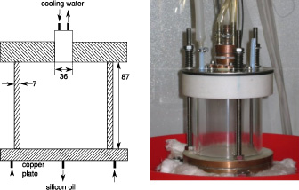
Schematic and photo of the cylindrical vessel for the modified Rayleigh–Bénard experiment.

Figure 1 shows the modified RB convection cell which consists of a cylindrical vessel with an inner diameter and also a height of 87 mm. The bottom of the vessel is heated homogeneously while the circular cooling zone on the top has a diameter of 36 mm. This corresponds to only 17% of the area that models the growing crystal. The boundary condition for the region that is not cooled on the top and at the side is adiabatic. The vessel is filled with the eutectic alloy GaInSn whose material parameters are given in [9]. The flow was first simulated for a temperature difference of 2.3 °C using the buoyantBoussinesqPimpleFoam solver of the finite volume library OpenFOAM over 3000 s [10], where no turbulence models were used. The simulated velocity served as basis for the computation of the induced magnetic field according to Eqs (1) and (2). The induced field has been computed by subsequently applying a horizontal and a vertical homogeneous primary field with $\mathbf{B}_{0,1}(\mathbf{r})=B_{0}∼\mathbf{e}_{x}$ and $\mathbf{B}_{0,2}(\mathbf{r})=B_{0}∼\mathbf{e}_{z}$ , where B ₀ = 3 mT, whereas only a single vertical primary field was employed for the measurements. The flow induced magnetic field was calculated at a distance of 36 mm from the fluid which resembles the smallest possible distance in the experimental setup [2]. Various sensor arrangements were investigated for a time-averaged and for a time-dependent flow.

Fig. 2.

Flow induced field $\mathbf{b}$ for a horizontal (a) and a vertical (b) primary field, and reconstruction (c) of the time-averaged large-scale circulation [2].

Table 1

Empirical correlation coefficient and rms error of the averaged flow with different sensor arrangements

Sensor arrangement	Correlation	Error
10 × 6	0.95	0.10
10 × 4	0.95	0.10
10 × 3	0.95	0.11
10 × 2	0.94	0.12
8 × 6	0.95	0.10
8 × 4	0.95	0.11
8 × 3	0.94	0.11
8 × 2	0.95	0.10
20 × 1	0.84	0.29
6 × 6	0.95	0.11
6 × 4	0.94	0.12
6 × 3	0.94	0.13
6 × 2	0.95	0.10
5 × 5	0.94	0.12
5 × 4	0.94	0.13
5 × 3	0.95	0.10
5 × 2	0.94	0.11

4. Stationary flow

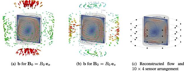
As a first assessment of the CIFT reconstruction, a time-averaged velocity field was used which was averaged over 500 s of the numerical simulation [2]. Figure 2(a) shows the time-averaged LSC which exhibits a flywheel structure. This velocity field served then as basis for the computation of the induced magnetic field according to Eqs (1) and (2). Figures 2(a) and (b) display the computed fields around the vessel for the two primary magnetic fields. These induced fields were then used, in turn, as input for the reconstruction of the velocity structure by solving the linear inverse problem. Figure 2(c) shows, for example, the reconstructed flow with a sensor arrangement of 10 sensors in azimuthal direction in 4 equally spaced planes over the height of the vessel. For reference, this arrangement is referred to as 10 × 4. In order to estimate the quality of the reconstruction, the empirical correlation coefficient and the root mean square (rms) error between the original and the reconstructed velocity field were calculated, giving values of 0.95 and 0.10, respectively. These values indicate a good agreement between the original and the reconstructed flow, and validate the procedure.

Various configurations with a varying number of sensors were subsequently considered to investigate the impact of the sensor arrangement on the quality of the reconstruction. Selected results are summarised in Table 1. The correlation coefficients and errors reveal that neither a reduced number of sensors in vertical nor in azimuthal direction seem to degrade the reconstruction significantly. The reason for this is most likely the relatively simple flow structure of the time-averaged LSC. Even a 20 × 1 configuration with 20 evenly distributed sensors along the azimuth in only a single plane at half of the height of the cylinder leads to reasonable results with a correlation coefficient of 0.84 and an error of 0.29, but with the an artificial vortex structure on the top of the cylinder. The appearance of this structure in this case results from the lack of necessary magnetic field data for the region [2]. 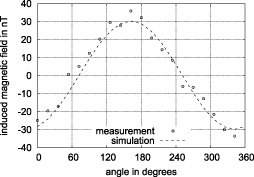A comparison of the simulated flow induced magnetic field for $\mathbf{B}_{0,z}$ to the measured flow induced magnetic field is shown in Fig. 3, where the simulated flow induced field was averaged over 500 s and the measured flow induced field over about 3 h. The measurement was performed with the 20 × 1 configuration, more details of the experimental setup are given in [2].

Fig. 3.

Measured and simulated flow induced field with primary field $\mathbf{B}_{0,z}$ .

5. Time dependent flow

The numerical flow simulation revealed that the time-dependent flow structure is by far more complex than the time-averaged flow and that phenomena such as sloshing and torsional modes become visible. In order to recover this behavior with CIFT, a reasonable azimuthal as well as vertical resolution of the flow induced magnetic field is required, but in practical applications the number of sensors is limited. It is therefore of interest, to arrange a given number of sensors in such a way that the resolution experiences a maximum. Three arrangements with 24 sensors, i.e. 12 × 2, 8 × 3, and 6 × 3, are considered for this task. A hypothetical sensor configuration with 7200 sensors in a 360 × 14 arrangement and with 1080 sensors above the top as well as 1080 sensors below the bottom of the cylinder serves as a reference case. Figure 4 shows the rms error and the correlation coefficient of the reconstructions with these four configurations. The results of the arrangements with 24 sensors differ only marginally, and also display no significant degradation of quality compared to the reference case. Considering that the flow induced magnetic field for a vertical primary field possesses its maximum at half of the height of the cylinder, the utilisation of the 8 × 3 arrangement is suggested as this arrangement is likely to be sensitive to global rotations of the LSC as well.

Fig. 4.

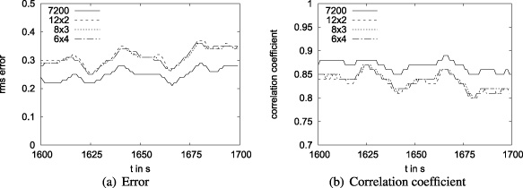
Error and correlation coefficient of the reconstruction with different sensor arrangements.

6. Conclusion

Various sensor arrangements have been examined to ensure a reliable reconstruction of typical flow features like sloshing and torsional modes of the LSC in a cylindrical RB configuration using CIFT. For the time-averaged flow, the quality of the reconstruction is not critically dependent on the number of sensors, where the rms error is approximately 0.1 and the correlation 0.95. The similar conclusion can be drawn for the number of sensors for the reconstruction of the time-dependent flow, but with a slightly increased error of approximately 0.3 and a decreased correlation of 0.8. Both measures for the quality of a reconstruction are in the typical range for CIFT. The simulations have been performed using a vertically and subsequently a horizontally directed primary field whereas the measurements have been carried out with a vertical field only. This limitation will be lifted in due course by utilising a second pair of coils for the generation of a horizontally directed field.

Footnotes

Acknowledgements

Financial support of the German Helmholtz Association in the framework of the Helmholtz-Alliance LIMTECH is gratefully acknowledged.

References

Stefani

Gundrum

and Gerbeth

, Contactless inductive flow tomography, Physical Review E 70 (2004), 056306(7p).

Wondrak

Pal

Stefani

Galindo

and Eckert

, Visualization of the global flow structure in a modified Rayleigh–Bénard setup using contactless inductive flow tomography, Flow Measurement and Instrumentation 62 (2018), 269–280.

Fünfschilling

and Ahlers

, Plume motion and large scale circulation in a cylindrical Rayleigh–Bénard cell, Phys. Rev. Lett. 92 (2004), 194502(4p).

Brown

and Ahlers

, The origin of oscillations of the large-scale circulation of turbulent Rayleigh–Bénard convection, J. Fluid Mech. 638 (2009), 383–400.

H.-D.

Zhou

S.-Q.

Chan

T.-S.

and Xia

K.-Q.

, Origin of temperature oscillation in turbulent thermal convection, Phys. Rev. Lett. 102 (2009), 044503(4p).

Hansen

P.C.

, Analysis of discrete ill-posed problems by means of the L-curve, Siam Review 34 (1992), 561–580.

Wondrak

Stefani

Gundrum

and Gerbeth

, Some methodological improvements of the contactless inductive flow tomography, Int. J. Appl. Electrom. 30 (2009), 255–264.

Ratajczak

Wondrak

and Stefani

, A gradiometric version of contactless inductive flow tomography: theory and first applications, Phil. Trans. T. Soc. A 374, 20150330.

Plevachuk

Sklyarchuk

Shevchenko

and Eckert

, Electrophysical and structure-sensitive properties of liquid Ga-In alloys, Int. J. Mater. Res. 106 (2015), 66–71.

10.

OpenFOAM Foundation: OpenFOAM - Free, open source software for CFD, http://openfoam.org, Version: 4.1 (2017).

Optimal sensor arrangement for Contactless Inductive Flow Tomography in the case of Rayleigh–Bénard convection

Abstract

Keywords

1. Introduction

2. Contactless Inductive Flow Tomography

Footnotes

Acknowledgements

References