Estimating the forcing function in a mechanical system by an inverse calibration method

Abstract

This article proposes and demonstrates a calibration-based integral formulation for resolving the forcing function in a mass–spring–damper system, given either displacement or acceleration data. The proposed method is novel in the context of vibrations, being thoroughly studied in the field of heat transfer. The approach can be expanded and generalized further to multi-variable systems associated with machine parts, vehicle suspensions, translational and rotational systems, gear systems, etc. when mathematically described by a system of constant property, linear, time-invariant ordinary differential equations. The analytic approach and subsequent numerical reconstruction of the forcing function is based on resolving a parameter-free inverse formulation for the equation(s) of motion. The calibration approach is formulated in the frequency domain and takes advantage of several observations produced by the dimensionality reduction leading to an algebratized system involving an input–output relationship and a transfer function possessing all the system parameters. The transfer function is eliminated in lieu of experimental data, from a calibration effort, thus leading to a reduction of systematic errors. These parameter-free, reduced systematic error aspects are the distinct and novel advantages of the proposed method. A first-kind Volterra integral equation is formed containing only the unknown forcing function and experimental data. As with all ill-posed problems, regularization must be introduced for system stabilization. A future-time technique is instituted for forming a family of predictions based on the chosen regularization parameter. The optimal regularization parameter is estimated using a combination of phase–plane analysis and cross-correlation principles. Finally, a numerical simulation is performed verifying the proposed approach.

Keywords

Inverse problem force identification integral equation regularization frequency domain cross-correlation

1. Introduction

Inverse problems naturally arise as one attempts to reconstruct the cause of a phenomenon from observables. These problems occur in many fields and contexts that include vibrations (Brownjohn et al., 2016; Chaigne, 2016; Jingjing, 2019; Vyas and Wicks, 2001; Woods and Lawrence, 1997) and heat transfer (Frankel and Keyhani, 2017; Frankel et al., 2013, 2017). Single equation and systems of equations are naturally formulated in the modeling of dynamic systems (Woods and Lawrence, 1997). Woods and Lawrence (1997) provide a wide array of examples involving machine parts, vehicle suspensions, translational and rotational systems, gear systems, etc. Most cases involve coupled linear ordinary differential equations describing the physical features of the model under consideration. This article, the first in a series, focuses on a single equation describing the motion of a forced mass–spring–damper (MSD) system. This example provides enough substance for describing the methodology and demonstrating its potential without undue, large-scale modeling. To illustrate the strength of the methodology, an additional example, based on machine part study taken from Woods and Lawrence (1997) (page 63), is also presented providing additional insight and clarity to the methodology’s features.

The calibration integral equation (Frankel and Keyhani, 2017; Frankel et al., 2013, 2017) was designed to resolve the so-called “inverse heat conduction problem” (Beck et al., 1985) associated with boundary condition reconstruction given in-depth measurements. In the context of vibrations, the inverse problem would be stated as “What is the forcing or driving function of a system given discretely measured temporal displacement, velocity, or acceleration data contaminated with noise?” Frankel and his colleagues (2013, 2017) have theorized and experimentally validated a novel parameter-free inverse methodology for the inverse heat conduction problem (Frankel and Keyhani, 2017; Frankel et al., 2013, 2017) based on partial differential equations (Sneddon, 1995).

The calibration integral equation approach is a potential substitute and successor for more traditional inverse methods employed in vibrations contexts. Some traditional methods in this context are the Kalman filtering scheme and the Tikhonov method (Hwang et al., 2009; Inoue et al., 2001; Jacquelin et al., 2003; Ma et al., 2003). The Kalman filtering scheme in the inverse vibrations problem context is a state-space analysis method. When employed by Ma et al., the method requires knowledge of system parameters, as opposed to the calibration integral equation. The Tikhonov method is the calibration integral equation’s direct competitor, as it does not require system parameter knowledge, takes advantage of Fourier transform and the frequency domain, and involves the convolution theorem. The Tikhonov method requires solving the deconvolution problem, which is ill-posed, using Tikhonov regularization (ridge regression). This regularization works by introducing an $l_{2}$ norm penalty, thus penalizing solution magnitude. The Tikhonov method is within a matrix paradigm, whereas the calibration integral equation uses a “time-marching” paradigm (Jacquelin et al., 2003; Frankel and Keyhani, 2017; Frankel et al., 2013, 2017). In practice, these paradigms are identical, but the resulting methods have their own resulting strengths. The Tikhonov method will be used as a comparative method in this article’s simulation results. Newer, sparce regularization methods are arriving which follow in the Tikhonov method’s footsteps. These methods use $l_{1}$ norm penalty (LASSO regression) to induce a sparce solution (Qiau et al., 2019).

The calibration integral equation is also closely related to solutions to moving force identification (MFI), another common inverse, ill-posed problem. MFI seeks to identify forces or loads on a bridge or beam. This is important information for analyzing structural dynamics. The similarity of MFI to the force reconstruction problem solved in this article is apparent. Many solutions to MFI stem from the Tikhonov method, and they rely upon singular value decomposition (SVD) and augments to SVD to resolve the ill-posed aspect of the problem (Chen et al., 2019a, 2019b). The generalized minimal residual algorithm has also been augmented and used to solve MFI (Chen et al., 2020).

Physical systems described by mathematical models possess inherent system parameters that are estimated either experimentally or theoretically, and thus possess uncertainties. No matter how accurate the numerical calculations are (based on a fixed set of input parameters), the results are subject to the inaccuracies perpetrated by the input parameters. These systematic errors can be removed using a calibration test where a highly accurate calibration source is required. Hence, the uncertainties in the system are associated with the input calibration source and measured observables. The question now arises “How can one systematically remove the parameters from the system?” This article describes a “systematic” approach for removing all properties from the mathematical formulation, and the resulting method is parameter-free and thus enjoys various strengths and reduced systematic error. Further, a unified methodology is proposed for resolving the forcing function of the inverse (ill-posed) problem based on a first-kind Volterra integral formulation (Kress, 1989; Linz, 1985; Wing, 1991).

Inverse problems are highly practical in engineering and the sciences. However, they possess numerous challenges due to their ill-posed mathematical structure where error amplification is rapidly observed when increasing the sampling rate. This article breaks the resolution process into three fundamental steps: reformulation, regularization, and regularization parameter selection. In a vibrations context, many formulations have been used to resolve inverse problems. Brownjohn et al. (2016), Chaigne (2016), Vyas and Wick (2001), and Jingjing (2019) each resolve an inverse problem of a vibrations system in different contexts with varying methods. Brownjohn et al. (2016) analyzed the vibrations of pedestrians on walking bridges and used acceleration measurements to generate frequency response functions and modal parameters. Chaigne (2016) resolved for the hammer force on a piano string from measured string velocity. Vyas and Wicks (2001) reconstructed blade forces on turbines from modal responses. Jingjing (2019) identified moving loads from response data using a local linear embedding algorithm. The methods employed in each of these studies either require that system parameters be known or require that they be estimated and used, thus introducing error and uncertainty.

All inverse problems require regularization for stability. Inverse problems are ill-posed which implies that measurements containing noise adversely affect stability, whereby skewing accuracy. The regularization methods applied in these studies (Brownjohn et al., 2016; Chaigne, 2016; Jingjing, 2019; Vyas and Wicks, 2001) are specific to the formulations used. In this article, the calibration integral equation approach is regularized using the future-time regularization concept (Beck et al., 1985; Frankel and Keyhani, 2017; Frankel et al., 2013, 2017). This method employs a future-time regularization parameter that must be chosen correctly for achieving accurate results. A popular approach for estimating the optimal regularization parameter is based on the so-called L-curve method (Lamm, 2000; Vogel, 1996) The validity of this method has been disputed by some (Vogel, 1996), and it was found to be inadequate for this article. Cross-correlation principles (Frankel and Keyhani, 2017; Frankel et al., 2017) have been demonstrated to work well for inverse heat conduction problems and chosen here as the means for extracting the optimal regularization parameter.

The MSD system leads to a common linear, time-invariant, second-order, initial-valued differential equation well-suited for demonstrating new concepts. Examples using MSD systems include seismic sensors, accelerometers, and car suspensions. A simple MSD model consists of a point mass connected to a relatively stationary surface by a spring and a damper. Energy is stored within the spring, and energy is dissipated by the damper. This causes the classic vibratory behavior of this system.

As stated above, the MSD system is a second-order system normally specified in terms of displacement. Thus, it can be modeled as a linear, time-invariant, second-order differential equation composed of three terms involving displacement, $x (t)$ ; a forcing or driver function, $f (t)$ ; and three system parameters. These system parameters are the mass of the system, $m_{0}$ ; the spring coefficient, $k_{0}$ ; and the damping coefficient, $c_{0}$ . Traditionally, the solution of this differential equation is sought for determining the displacement, $x (t)$ , when given $f (t)$ , $m_{0}$ , $k_{0}$ , and $c_{0}$ . However, this note considers the inverse problem involving the estimation of $f (t)$ , given only a measurement of either the displacement or acceleration, $a (t)$ . The approach introduced in this note also eliminates the necessity of knowing the values of the system parameters, $m_{0}$ , $k_{0}$ , and $c_{0}$ .

2. Formulation

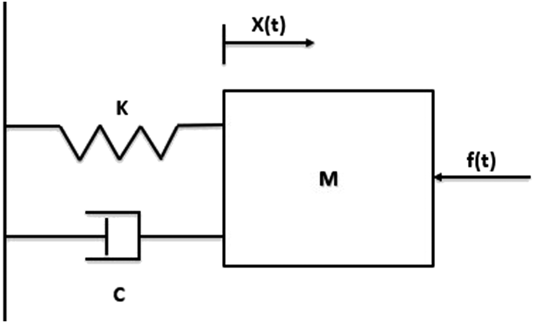
To place physical context to this formulation, consider the MSD system displayed in Figure 1. Note that the MSD system is merely a convenient example for demonstrating the procedures and capabilities of this formulation. In this situation, $x (t)$ is displacement of the mass relative to the datum, $v (t) = d x / d t (t)$ represents the velocity of the mass, and $a (t) = d^{2} x / d t^{2} (t)$ represents the acceleration of the mass.

Figure 1.

Mass–spring–damper system.

The resulting equation of motion is given as

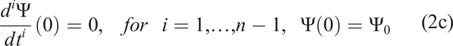
\begin{matrix} m_{o} \frac{d^{2} x}{d t^{2}} (t) + c_{o} \frac{d x}{d t} (t) + k_{o} x (t) = f (t), t \geq 0 \end{matrix}

(1a)

Subject to the trivial initial conditions

\begin{matrix} x (0) = x_{0} = 0, \frac{d x}{d t} (0) = x_{0}^{'} = 0 \end{matrix}

(1b-c)

In most investigations, the solution to equation (1a), subject to the initial conditions displayed in equations (1b–c), is sought when provided the coefficients $m_{0}$ , $k_{0}$ , and $c_{0}$ , and forcing function, $f (t)$ . However, in many experimental investigations, either the coefficients are unknown and/or the forcing function must be reconstructed. This reversal leads to the inverse problem which possesses its own unique difficulties. The question arises “Can we estimate the forcing function in a manner that substantially reduces systematic errors introduced through the coefficients $m_{0}$ , $k_{0}$ , and $c_{0}$ ?” Clearly, if given $m_{0}$ , $k_{0}$ , and $c_{0}$ , then theoretically one can recover the forcing function by making measurements in $x (t)$ . These discrete data contain measurement errors that can play havoc (unless regularized by some means) on higher-time derivatives of the dependent variable described in equation (1a).

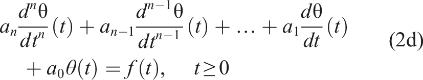
To motivate this study and display the vast utility of the calibration integral equation approach, consider an $n^{t h}$ order ordinary differential equation of some variable $Ψ$

\begin{matrix} a_{n} \frac{d^{n} Ψ}{d t^{n}} (t) + a_{n - 1} \frac{d^{n - 1} Ψ}{d t^{n - 1}} (t) + \dots + a_{1} \frac{d Ψ}{d t} (t) + a_{0} Ψ (t) = f (t), t \geq 0 \end{matrix}

(2a)

and initial conditions

\begin{matrix} Ψ (0) = Ψ_{0} \end{matrix}

(2b)

\begin{matrix} \frac{d^{i} Ψ}{d t^{i}} (0) = 0, f o r i = 1, \dots, n - 1, Ψ (0) = Ψ_{0} \end{matrix}

(2c)

where

a_{i}

are constants. Notice that the MSD system, equation (1a), is merely equation (2a) with

n = 2,

a_{2} = m_{0}

a_{1} = c_{0}

a_{0} = k_{0}

, and

Ψ_{0} = 0

. Equation (2a) can be simplified with respect to the initial condition in equation (2b) to yield

\begin{matrix} a_{n} \frac{d^{n} θ}{d t^{n}} (t) + a_{n - 1} \frac{d^{n - 1} θ}{d t^{n - 1}} (t) + \dots + a_{1} \frac{d θ}{d t} (t) + a_{0} θ (t) = f (t), t \geq 0 \end{matrix}

(2d)

with

θ

defined as

\begin{matrix} θ (t) = Ψ (t) - Ψ_{0} \end{matrix}

(2e)

This simplification reduces the initial conditions to a trivial case.

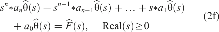
The normal process for arriving at a solution for $θ (t)$ is to take the Laplace transform of equation (2d)

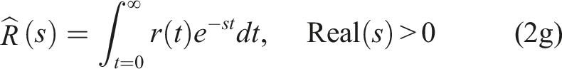
\begin{matrix} s^{n} * a_{n} \hat{θ} (s) + s^{n - 1} * a_{n - 1} \hat{θ} (s) + \dots + s * a_{1} \hat{θ} (s) + a_{0} \hat{θ} (s) = \hat{F} (s), Real (s) \geq 0 \end{matrix}

(2f)

where the Laplace transform (Sneddon, 1995) is defined as

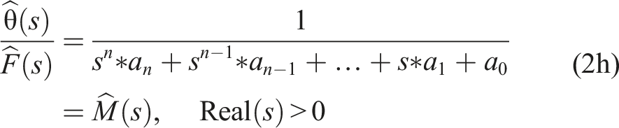
\begin{matrix} \hat{R} (s) = \int_{t = 0}^{\infty} r (t) e^{- s t} d t, Real (s) > 0 \end{matrix}

(2g)

for real function

r (t)

. Equation (2f) can be placed into an output to input form. Doing so produces the transfer function

\hat{M} (s)

given by

\begin{matrix} \frac{\hat{θ} (s)}{\hat{F} (s)} = \frac{1}{s^{n} * a_{n} + s^{n - 1} * a_{n - 1} + \dots + s * a_{1} + a_{0}} = \hat{M} (s), Real (s) > 0 \end{matrix}

(2h)

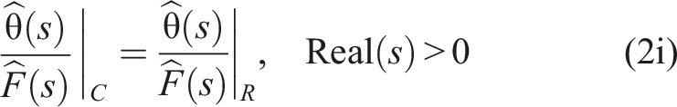
Because the system is linear and time invariant, the transfer function, $\hat{M} (s)$ , can be eliminated in terms of a similar ratio involving consecutive experimental tests, which assumes that the system parameters remain constant among all future tests (which is the bedrock of most studies). That is, using test one measurements involving an imposed driver, $f_{c} (t)$ , and measured $θ_{c} (t)$ , we can eliminate the transfer function in the frequency domain. This portion of the test program is called the calibration run and is normally performed in a laboratory high-quality test environment. In this way, the measurements are considered benchmark accurate. Taking the system to the field and performing other tests now provides a means for estimating the reconstruction or field test. With this understanding, equation (2c) can be expressed as

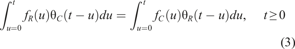
\begin{matrix} {\frac{\hat{θ} (s)}{\hat{F} (s)} |}_{C} = {\frac{\hat{θ} (s)}{\hat{F} (s)} |}_{R}, Real (s) > 0 \end{matrix}

(2i)

where “C” represents calibration and “R” represents reconstruction cases. Next, we cross multiply and invert with the aid of the convolution theorem (Sneddon, 1995) to acquire

\begin{matrix} \int_{u = 0}^{t} f_{R} (u) θ_{C} (t - u) d u = \int_{u = 0}^{t} f_{C} (u) θ_{R} (t - u) d u, t \geq 0 \end{matrix}

(3)

which is a first-kind Volterra integral equation for

f_{R} (t)

when given measured

f_{C} (t)

, measured

θ_{C} (t)

, and measured

θ_{R} (t)

from a second or field test. We refer to this formulation as the calibration integral equation. Notice the absence of system parameters in this formulation. This process substantially reduces systematic errors but increases the significance of performing a high-quality calibration campaign. Equation (3) now places the analysis into an ill-posed integral framework for the recovery of

f_{R} (t)

. As noted previously, the present first-kind Volterra integral equation for

f_{R} (t)

is highly ill-posed and any noise in the data is expected to amplify in the reconstruction of

f_{R} (t)

. This effect is exacerbated as the sampling rate increases. As with all ill-posed problems, regularization must be introduced for a meaningful approximation to be successfully recovered.

As noted previously, this method is currently employed in the field of heat transfer ( Frankel and Keyhani, 2017; Frankel et al., 2013, 2017). Later in this article, a similar analysis is performed on the MSD system expressed in terms of the acceleration of the system.

3. Regularization by future time and numerical discretization using displacement data

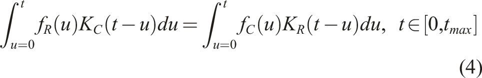
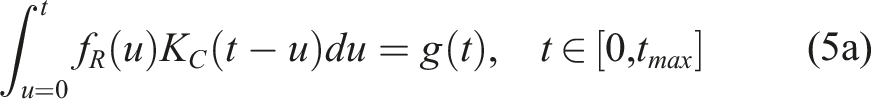
Regularization must be introduced to stabilize the reconstruction of $f_{R} (t)$ (Beck et al., 1985; Frankel and Keyhani, 2017; Frankel et al., 2013, 2017). The method proposed here is based on a future-time concept (Beck et al., 1985; Frankel and Keyhani, 2017; Frankel et al., 2013, 2017). In an actual experiment, the time domain is finite, and the data are not continuous. Further, the data contain noise. Let the end of the data collection period be denoted as $t = t_{m a x}$ . However, it is quite convenient to derive the desired method for reconstructing $f_{R} (t)$ in the continuous variable sense, and then discretize the final form in preparation of experimental data. Rewriting equation (3) in a conventional form produces

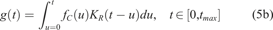
\begin{matrix} \int_{u = 0}^{t} f_{R} (u) K_{C} (t - u) d u = \int_{u = 0}^{t} f_{C} (u) K_{R} (t - u) d u, t \in [0, t_{m a x}] \end{matrix}

(4)

where K_C and K_R are called the kernels. In this statement,

f_{C}

K_{C}

, and

K_{R}

are known. Thus, the right-hand side is a known function of time that can alternatively be expressed in standard first-kind Volterra (Linz, 1985) form as

\begin{matrix} \int_{u = 0}^{t} f_{R} (u) K_{C} (t - u) d u = g (t), t \in [0, t_{m a x}] \end{matrix}

(5a)

with the driving function,

g (t)

, expressed as

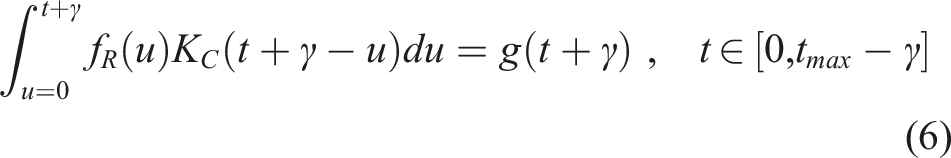
\begin{matrix} g (t) = \int_{u = 0}^{t} f_{C} (u) K_{R} (t - u) d u, t \in [0, t_{m a x}] \end{matrix}

(5b)

To begin the future-time method, time is advanced as $t \to t + γ$ , with $γ \geq 0$ in equation (5a) where the future-time parameter is denoted as $γ$ . Performing this time advancement produces

\begin{matrix} \int_{u = 0}^{t + γ} f_{R} (u) K_{C} (t + γ - u) d u = g (t + γ), t \in [0, t_{m a x} - γ] \end{matrix}

(6)

Observe that the resolvable time domain for the prediction space of $f_{R} (t)$ is reduced to $t_{m a x} - γ$ .

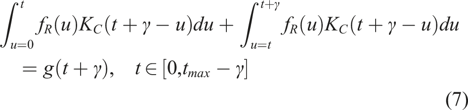
From basic calculus, the left-hand side of equation (6) can alternatively be expressed as

\int_{u = 0}^{t} f_{R} (u) K_{C} (t + γ - u) d u + \int_{u = t}^{t + γ} f_{R} (u) K_{C} (t + γ - u) d u = g (t + γ), t \in [0, t_{m a x} - γ]

(7)

\int_{u = 0}^{t} f_{R} (u) K_{C} (t + γ - u) d u + f_{R} (t) \int_{u = t}^{t + γ} K_{C} (t + γ - u) d u \approx g (t + γ), t \in [0, t_{m a x} - γ]

(8a)

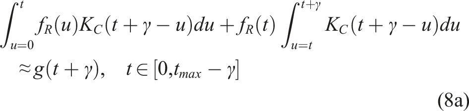
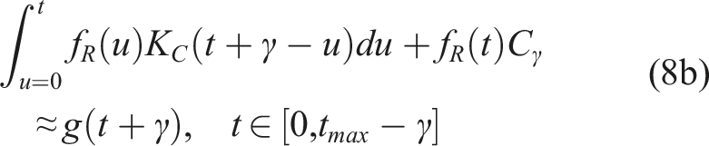
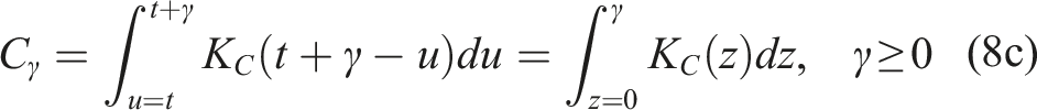
where it is assumed that

f_{R} (u) = f_{R} (t)

u \in [t, t + γ]

. This implies that

γ

is small for this assumption to hold. This is the first approximation introduced into the predictive process for recovering or resolving

f_{R} (t)

. Notice that equality is lost in equation (8a) by this process. Before proceeding further, observe that equation (8a) can be simplified by defining the constant

C_{γ}

such that

\begin{matrix} \int_{u = 0}^{t} f_{R} (u) K_{C} (t + γ - u) d u + f_{R} (t) C_{γ} \approx g (t + γ), t \in [0, t_{m a x} - γ] \end{matrix}

(8b)

where

\begin{matrix} C_{γ} = \int_{u = t}^{t + γ} K_{C} (t + γ - u) d u = \int_{z = 0}^{γ} K_{C} (z) d z, γ \geq 0 \end{matrix}

(8c)

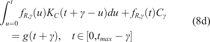
To recapture the equal sign in equations (8b), a notational change is required. Thus, we express equation (8b) as

\begin{matrix} \int_{u = 0}^{t} f_{R, γ} (u) K_{C} (t + γ - u) d u + f_{R, γ} (t) C_{γ} = g (t + γ), t \in [0, t_{m a x} - γ] \end{matrix}

(8d)

where

f_{R, γ} (t) \approx f_{R} (t)

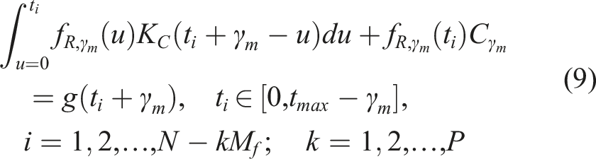
. Equation (8d) is representative of a second-kind Volterra integral equation which possesses better stability characteristics than first-kind equations for sufficiently large

C_{γ} .

A carefully defined approximation thread is now being constructed in the model and computational processes. At this juncture, we now move from the continuous variable approach to a discrete or experimental viewpoint. That is, let

t \to t_{i}

, where

t_{i} = i Δ t

with

i = 0,1, \dots, N

and

Δ t = t_{m a x} / N

. The sampling frequency becomes

f = 1 / Δ t

with the uniform sampling width of

Δ t

. Further, let the continuous future-time parameter concurrently be considered as a discrete variable and given by

γ \to γ_{m} = m Δ t = k M_{f} Δ t

, where

M_{f}

is a convenient multiplication factor needed in generating a family of predictions,

k

is an index integer, and

m

is the future-time parameter index. This three-part formulation of

γ_{m}

is convenient for iterating through future-time parameters efficiently. One sets

M_{f}

and iterates

k = 1,2, \dots P

to form a set of future-time parameter indices,

{M_{f}, 2 M_{f}, \dots P M_{f}}

. The optimal parameter is then chosen from that set. Thus, a discrete spectrum of values exists describing the future-time regularization parameter. Observe that the discrete future-time parameter is based on the sampling frequency for convenience. With this operation a family of predictions for

f_{R, γ} (t)

, namely,

f_{R, γ_{m}} (t)

, is produced. Correspondingly, equation (8d) is now expressed as

\begin{matrix} \int_{u = 0}^{t_{i}} f_{R, γ_{m}} (u) K_{C} (t_{i} + γ_{m} - u) d u + f_{R, γ_{m}} (t_{i}) C_{γ_{m}} = g (t_{i} + γ_{m}), t_{i} \in [0, t_{m a x} - γ_{m}] \end{matrix}, i = 1,2, \dots, N - k M_{f}; k = 1,2, \dots, P

(9)

where P is the user chosen maximum number of predictions in the family. Equation (9) is expressed in a regional sense corresponding to an experimentalist view as

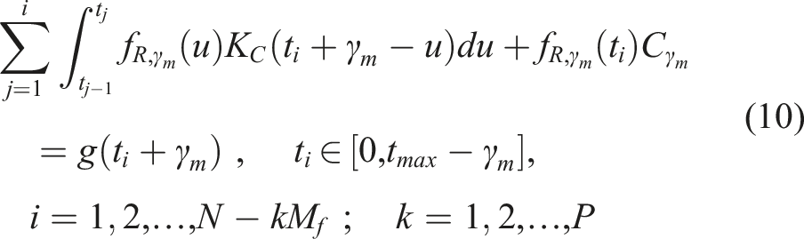
\begin{matrix} \begin{array}{l} \sum_{j = 1}^{i} \int_{t_{j - 1}}^{t_{j}} f_{R, γ_{m}} (u) K_{C} (t_{i} + γ_{m} - u) d u + f_{R, γ_{m}} (t_{i}) C_{γ_{m}} \\ = g (t_{i} + γ_{m}), t_{i} \in [0, t_{m a x} - γ_{m}], i = 1,2, \dots, N - k M_{f}; k = 1,2, \dots, P \end{array} \end{matrix}

(10)

The i^th term of this summation can be extracted as

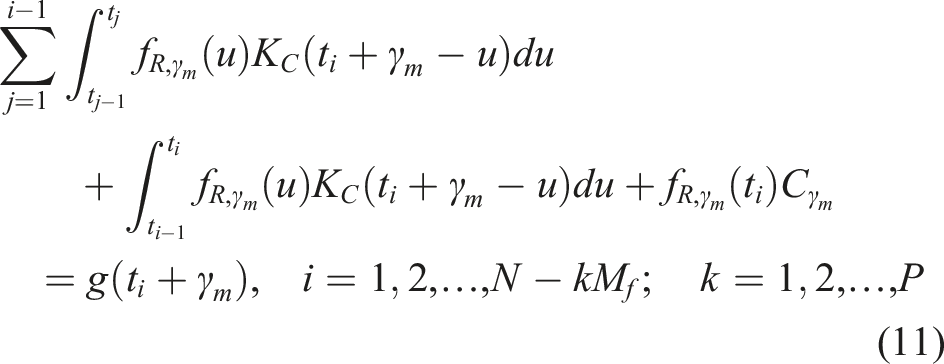
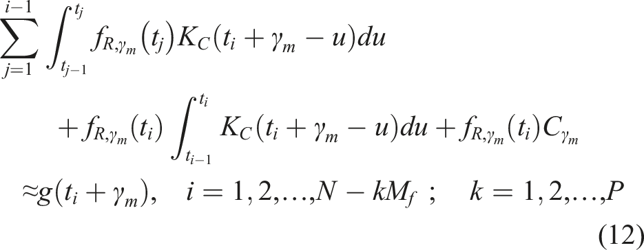
\begin{array}{l} \sum_{j = 1}^{i - 1} \int_{t_{j - 1}}^{t_{j}} f_{R, γ_{m}} (u) K_{C} (t_{i} + γ_{m} - u) d u + \int_{t_{i - 1}}^{t_{i}} f_{R, γ_{m}} (u) K_{C} (t_{i} + γ_{m} - u) d u + f_{R, γ_{m}} (t_{i}) C_{γ_{m}} \\ = g (t_{i} + γ_{m}), i = 1,2, \dots, N - k M_{f}; k = 1,2, \dots, P \end{array}

(11)

Introducing a product-rule integration (Linz, 1985) for the preceding panel of the i^th value of the unknown function where $f_{R, γ_{m}} (t)$ is held constant on $t \in [t_{i - 1}, t_{i}]$ yields

\begin{array}{l} \sum_{j = 1}^{i - 1} \int_{t_{j - 1}}^{t_{j}} f_{R, γ_{m}} (t_{j}) K_{C} (t_{i} + γ_{m} - u) d u + f_{R, γ_{m}} (t_{i}) \int_{t_{i - 1}}^{t_{i}} K_{C} (t_{i} + γ_{m} - u) d u + f_{R, γ_{m}} (t_{i}) C_{γ_{m}} \\ \approx g (t_{i} + γ_{m}), i = 1,2, \dots, N - k M_{f}; k = 1,2, \dots, P \end{array}

(12)

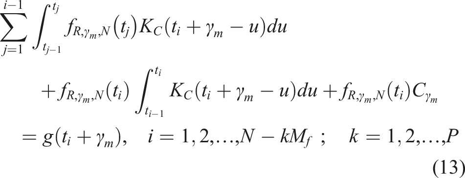
Notice that equality is lost in equation (12). To regain the equality, let $f_{R, γ_{m}, N} (t) \approx f_{R, γ_{m}} (t) \approx f_{R} (t)$ . Thereby, equation (13) becomes

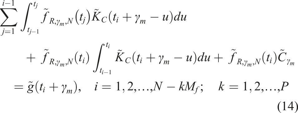
\begin{array}{l} \sum_{j = 1}^{i - 1} \int_{t_{j - 1}}^{t_{j}} f_{R, γ_{m}, N} (t_{j}) K_{C} (t_{i} + γ_{m} - u) d u + f_{R, γ_{m}, N} (t_{i}) \int_{t_{i - 1}}^{t_{i}} K_{C} (t_{i} + γ_{m} - u) d u + f_{R, γ_{m}, N} (t_{i}) C_{γ_{m}} \\ = g (t_{i} + γ_{m}), i = 1,2, \dots, N - k M_{f}; k = 1,2, \dots, P \end{array}

(13)

At this junction in the derivation, all discrete data are assumed errorless. In fact, these data contain noise and the formulation should display these errors in the measurements. The tilde-notation “∼” is used to identify noise in the datasets. Thus, equation (13) becomes

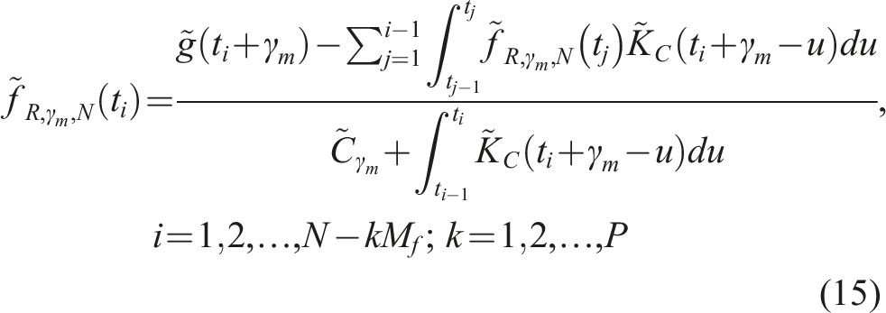
\begin{array}{l} \sum_{j = 1}^{i - 1} \int_{t_{j - 1}}^{t_{j}} {\tilde{f}}_{R, γ_{m}, N} (t_{j}) {\tilde{K}}_{C} (t_{i} + γ_{m} - u) d u + {\tilde{f}}_{R, γ_{m}, N} (t_{i}) \int_{t_{i - 1}}^{t_{i}} {\tilde{K}}_{C} (t_{i} + γ_{m} - u) d u + {\tilde{f}}_{R, γ_{m}, N} (t_{i}) {\tilde{C}}_{γ_{m}} \\ = \tilde{g} (t_{i} + γ_{m}), i = 1,2, \dots, N - k M_{f}; k = 1,2, \dots, P \end{array}

(14)

The growing approximation thread is now defined through ${\tilde{f}}_{R, γ_{m}, N} (t) \approx f_{R, γ_{m}, N} (t) \approx f_{R, γ_{m}} (t) \approx f_{2} (t)$ . Next, we algebraically solve for ${\tilde{f}}_{R, γ_{m}, N} (t_{i})$ to arrive at

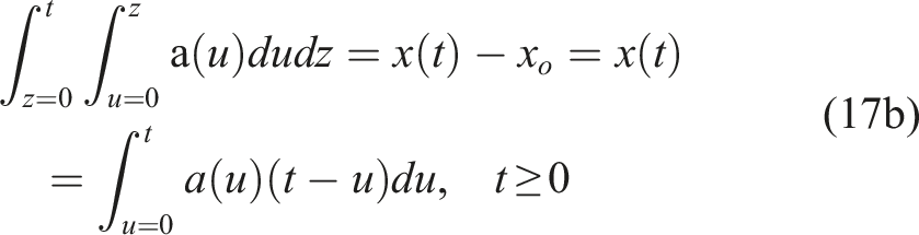
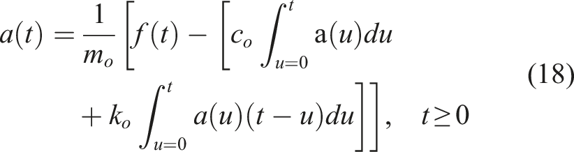
\begin{matrix} {\tilde{f}}_{R, γ_{m}, N} (t_{i}) = \frac{\tilde{g} (t_{i} + γ_{m}) - \sum_{j = 1}^{i - 1} \int_{t_{j - 1}}^{t_{j}} {\tilde{f}}_{R, γ_{m}, N} (t_{j}) {\tilde{K}}_{C} (t_{i} + γ_{m} - u) d u}{{\tilde{C}}_{γ_{m}} + \int_{t_{i - 1}}^{t_{i}} {\tilde{K}}_{C} (t_{i} + γ_{m} - u) d u} \end{matrix}, i = 1,2, \dots, N - k M_{f}; k = 1,2, \dots, P

(15)

Equation (15) leads to a time marching numerical implementation that retains physical causality. Observe that for a MSD system, the present formulation is based on measured displacement data. In many applications, acceleration data can be used based on an accelerometer (i.e., $a (t) = d^{2} x / d t^{2}$ ). The next section provides the fundamental steps for using acceleration data in place of displacement data when working with a MSD system.

4. MSD system using acceleration data

Recall equations (1a–c) and the physical configuration describing the mathematical formulation, namely, Figure 1. Let $\ddot{x} (t)$ be defined as $a (t)$ and for the moment isolate this definition of acceleration therefore

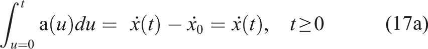
\begin{matrix} a (t) = \ddot{x} (t) = \frac{1}{m_{o}} [f (t) - [c_{o} \dot{x} (t) + k_{o} x (t)]], t \geq 0 \end{matrix}

(16)

Integrating the acceleration yields

\begin{matrix} \int_{u = 0}^{t} a (u) d u = \dot{x} (t) - {\dot{x}}_{0} = \dot{x} (t), t \geq 0 \end{matrix}

(17a)

from equation (1c). Integrating equation (17a) produces

\begin{matrix} \int_{z = 0}^{t} \int_{u = 0}^{z} a (u) d u d z = x (t) - x_{o} = x (t) = \int_{u = 0}^{t} a (u) (t - u) d u, t \geq 0 \end{matrix}

(17b)

which uses equation (1b) and realizing that integration on the triangle was produced. Combining equations (16) and (17a-b) produces

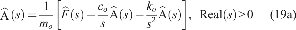
\begin{matrix} a (t) = \frac{1}{m_{o}} [f (t) - [c_{o} \int_{u = 0}^{t} a (u) d u + k_{o} \int_{u = 0}^{t} a (u) (t - u) d u]], t \geq 0 \end{matrix}

(18)

Taking the Laplace transform of equation (18) yields

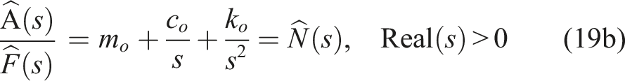
\begin{matrix} \hat{A} (s) = \frac{1}{m_{o}} [\hat{F} (s) - \frac{c_{o}}{s} \hat{A} (s) - \frac{k_{o}}{s^{2}} \hat{A} (s)], Real (s) > 0 \end{matrix}

(19a)

which can be expressed as the ratio of output to input as

\begin{matrix} \frac{\hat{A} (s)}{\hat{F} (s)} = m_{o} + \frac{c_{o}}{s} + \frac{k_{o}}{s^{2}} = \hat{N} (s), Real (s) > 0 \end{matrix}

(19b)

with

\hat{N} (s)

being the transfer function associated with the acceleration formulation. Thus, using a measured acceleration in a MSD system permits the identical calibration integral equation approach for determining the forcing function

f_{R} (t)

as described when using displacement data.

Hence, the next logical question arises “How does one identify the optimal regularization parameter?” In fact, this is the major quest for all inverse problems and regularization methods.

5. Optimal future-time parameter selection

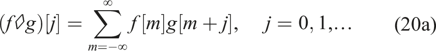
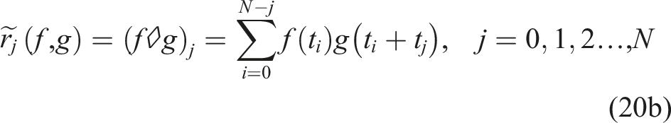
This section describes an approach for estimating the optimal future-time parameter, $γ_{m}$ . The remainder of this note will use the displacement formulation. Notice that when $γ_{m} = 0$ in equation (8d), the original Volterra integral equation of the first kind is recovered. Thus, if $γ_{m}$ is sufficiently small then stability will remain a concern. Alternatively, if $γ_{m}$ is too large then the prediction will become oversmoothed, and accuracy will be reduced. Thus, it is necessary to estimate a minimum error producing $γ_{m}$ . One common method for choosing this optimal parameter is the L-curve method (Lamm, 2000). This method was quickly found to be insufficient for the task, and this finding supports other findings involving the non-convergence of this method (Vogel, 1996).The method used to estimate the optimal future-time parameter is based on phase–plane analysis and cross-correlation principles (Frankel and Keyhani, 2017). Cross correlation is a common tool in signal processing. It measures the similarity between two signals (Oppenheim and Schafer, 1975). The traditional definition of cross correlation for two discrete and infinite data sets $f$ and $g$ with discrete lag $j$ is

\begin{matrix} (f ◇ g) [j] = \sum_{m = - \infty}^{\infty} f [m] g [m + j], j = 0,1, \dots \end{matrix}

(20a)

For discrete data collected with a fixed sampling width $Δ t$ , equation (20a) must change to reflect this reduction in data. The datasets are denoted $f (t_{i})$ and $g (t_{i})$ , where $t_{i} = i Δ t$ and $i = 0,1, \dots, N .$ Equation (20a) becomes

\begin{matrix} \tilde{r_{j}} (f, g) = {(f ◇ g)}_{j} = \sum_{i = 0}^{N - j} f (t_{i}) g (t_{i} + t_{j}), j = 0,1,2 \dots, N \end{matrix}

(20b)

The similarity of the two datasets $f$ and $g$ is denoted by the size of $\tilde{r_{j}}$ . Larger values of $\tilde{r_{j}}$ imply great similarity, whereas smaller values indicate less similarity. A sufficiently small cross correlation would imply near orthogonality between the two datasets.

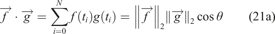
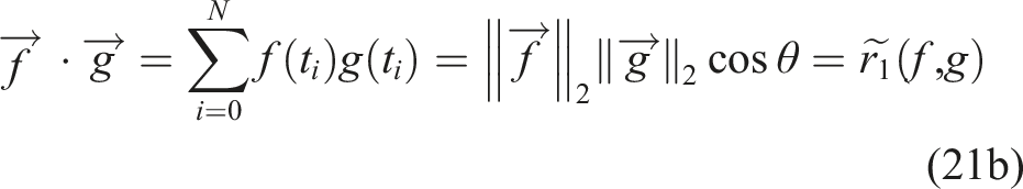
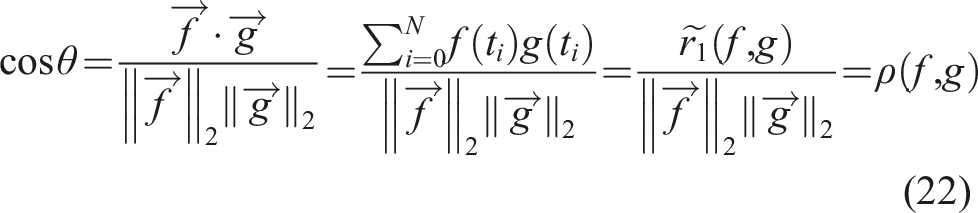
When applied to the future-time regularization scheme, the lag associated with cross correlation is set to zero, $j = 0$ (the reader is referred to Ref. [7], for further explanation). When setting $j = 0$ , cross correlation is visually similar to the dot product or inner product. A dataset, $f$ , with $(N + 1)$ points is equivalent to a $(N + 1)$ -dimensional vector, $\vec{f}$ . Thus, (Frankel and Keyhani, 2017)

\vec{f} \cdot \vec{g} = \sum_{i = 0}^{N} f (t_{i}) g (t_{i}) = {‖ \vec{f} ‖}_{2} {‖ \vec{g} ‖}_{2} \cos θ

(21a)

where

θ

is the angle subtended between the two vectors. The parallel between the dot product and cross correlation is evident from equation (21a). In fact

\begin{matrix} \vec{f} \cdot \vec{g} = \sum_{i = 0}^{N} f (t_{i}) g (t_{i}) = {‖ \vec{f} ‖}_{2} {‖ \vec{g} ‖}_{2} \cos θ = \tilde{r_{1}} (f, g) \end{matrix}

(21b)

where the vector two-norm is

{‖ \vec{f} ‖}_{2} = \sqrt{\sum_{i = 0}^{N} f^{2} (t_{i})}

. The cross correlation can be normalized to yield

\begin{matrix} \cos θ = \frac{\vec{f} \cdot \vec{g}}{{‖ \vec{f} ‖}_{2} {‖ \vec{g} ‖}_{2}} = \frac{\sum_{i = 0}^{N} f (t_{i}) g (t_{i})}{{‖ \vec{f} ‖}_{2} {‖ \vec{g} ‖}_{2}} = \frac{\tilde{r_{1}} (f, g)}{{‖ \vec{f} ‖}_{2} {‖ \vec{g} ‖}_{2}} = ρ (f, g) \end{matrix}

(22)

where

ρ

is the cross-correlation coefficient. This coefficient will be a real number,

ρ \in [- 1,1]

. A cross-correlation coefficient approaching unity implies that the vectors are highly correlated, or that the two datasets are similar. A coefficient approaching zero implies that the two datasets are not similar and nearly orthogonal.

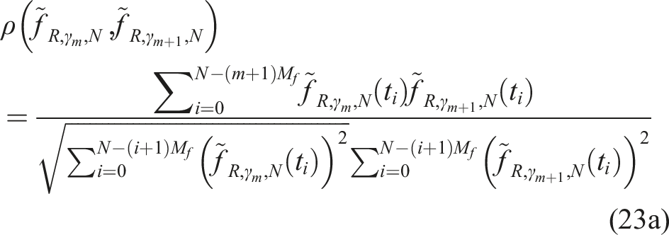
To find the optimal future-time parameter, a set (m, m+1) of successive parameters are used. The cross-correlation parameter is calculated for two successive reconstructions and the numerical derivative of the two reconstructions. Mathematically, we express these as

\begin{matrix} ρ ({\tilde{f}}_{R, γ_{m}, N}, {\tilde{f}}_{R, γ_{m + 1}, N}) = \frac{\sum_{i = 0}^{N - (m + 1) M_{f}} {\tilde{f}}_{R, γ_{m}, N} (t_{i}) {\tilde{f}}_{R, γ_{m + 1}, N} (t_{i})}{\sqrt{\sum_{i = 0}^{N - (i + 1) M_{f}} {({\tilde{f}}_{R, γ_{m}, N} (t_{i}))}^{2} \sum_{i = 0}^{N - (i + 1) M_{f}} {({\tilde{f}}_{R, γ_{m + 1}, N} (t_{i}))}^{2}}} \end{matrix}

(23a)

\begin{matrix} \dot{ρ} ({\dot{\tilde{f}}}_{R, γ_{m}, N}, {\dot{\tilde{f}}}_{R, γ_{m + 1}, N}) = \frac{\sum_{i = 0}^{N - (i + 1) M_{f}} {\dot{\tilde{f}}}_{R, γ_{m}, N} (t_{i}) {\dot{\tilde{f}}}_{R, γ_{m + 1}, N} (t_{i})}{\sqrt{\sum_{i = 0}^{N - (i + 1) M_{f}} {({\dot{\tilde{f}}}_{R, γ_{m}, N} (t_{i}))}^{2} \sum_{i = 0}^{N - (i + 1) M_{f}} {({\dot{\tilde{f}}}_{R, γ_{m + 1}, N} (t_{i}))}^{2}}} \end{matrix}

(23b)

where

M_{f}

is a multiplication factor. As

ρ ({\tilde{f}}_{R, γ_{m}, N}, {\tilde{f}}_{R, γ_{m + 1}, N}) \to 1

, the reconstruction is known to display a converging characteristic, but, as

\dot{ρ} ({\dot{\tilde{f}}}_{R, γ_{m}, N}, {\dot{\tilde{f}}}_{R, γ_{m + 1}, N}) \to 1

, the rate predictions produce oversmoothed predictions. Thus, the desirable future-time parameter has

ρ ≅ 1

; however, one should avoid driving

\dot{ρ} \to 1

. It is well-known that the time derivative of the data drives the stability of the system.

6. Versatility

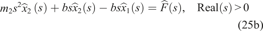
Before providing the last part of the roadmap, that is, results, a brief diversion is offered illustrating the power of reformulation. By way of a simple example taken from Woods and Lawrence (1997), pp. 63–65, Figures 3.12-3.14 which involves a machine part modeled as

\begin{matrix} m_{1} {\ddot{x}}_{1} (t) + b {\dot{x}}_{1} (t) - b {\dot{x}}_{2} (t) + k x_{1} (t) = 0 \end{matrix}

(24a)

\begin{matrix} m_{2} {\ddot{x}}_{2} (t) + b {\dot{x}}_{2} (t) - b {\dot{x}}_{1} (t) = F (t), t \geq 0 \end{matrix}

(24b)

Subject to trivial initial conditions, $x_{n}^{(j)} = 0, n = 1,2; j = 0, 1$ and requiring the specification of four physical parameters. Equations (24a and 24b) describe the equations of motion for this two-mass problem [5, p: 64]. This mathematical model describes a machine part with upper mass, $m_{2}$ , that ”slides” along a lubricated surface interfacing a lower mass, $m_{1}$ . The lower mass is a spring connected to a fixed base. A forcing function, $F (t)$ , drives the operation of the upper mass, $m_{2}$ . Unlike the approach taken in Woods and Lawrence (1997), here we directly take the Laplace transform of equations (24a and 24b) to get

\begin{matrix} m_{1} s^{2} {\hat{x}}_{1} (s) + b s {\hat{x}}_{1} (s) - b s {\hat{x}}_{2} (s) + k {\hat{x}}_{1} (s) = 0 \end{matrix}

(25a)

\begin{matrix} m_{2} s^{2} {\hat{x}}_{2} (s) + b s {\hat{x}}_{2} (s) - b s {\hat{x}}_{1} (s) = \hat{F} (s), Real (s) > 0 \end{matrix}

(25b)

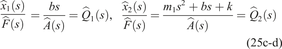
which incorporates the trivial initial conditions. Expressing equations (25a and 25b) in a matrix form allowing us to solve for

{\hat{x}}_{1} (s), {\hat{x}}_{2} (s)

. As the last step, we express the output to input ratio in the frequency domain as

\begin{matrix} \frac{{\hat{x}}_{1} (s)}{\hat{F} (s)} = \frac{b s}{\hat{A} (s)} = {\hat{Q}}_{1} (s), \frac{{\hat{x}}_{2} (s)}{\hat{F} (s)} = \frac{m_{1} s^{2} + b s + k}{\hat{A} (s)} = {\hat{Q}}_{2} (s) \end{matrix}

(25c-d)

\begin{matrix} \hat{A} (s) = m_{1} m_{2} s^{4} + (m_{1} + m_{2}) b s^{3} + k m_{2} s^{2} + k b s, Real (s) > 0 \end{matrix}

(25e)

where

{\hat{Q}}_{1} (s)

and

{\hat{Q}}_{2} (s)

are transfer functions for this system. This now places the formulation into an equivalent starting point, equation (2h) for the methodology using displacement data. Again, this approach does not require any physical properties to be specified. Finally, observable (measurable) displacement data based on either mass one or mass two can be used for estimating

F (t)

Appendix A contains a brief proof of concept simulation of this versatility.

7. Results

This section presents numerical results for a MSD system based on displacement datasets. To test the scheme, the MSD system parameters were chosen as $m_{o} = 0.05 (kg)$ , $c_{o} = 30 (Ns / m)$ , and $k_{o} = 5000 (N / m)$ . With these system parameters, the motion of the system on $t \in [0,4] s$ was analytically found for the two forcing functions (in Newtons)

\begin{matrix} f_{1} (t) = 50 \sin (5 π t) + 20 \sin (20 π t) \end{matrix}

(26a)

\begin{matrix} f_{2} (t) = 30 (1 - U (t - 1)) \end{matrix}

(26b)

where

U (t)

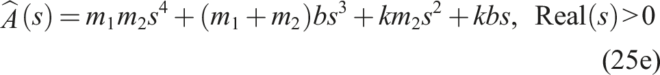
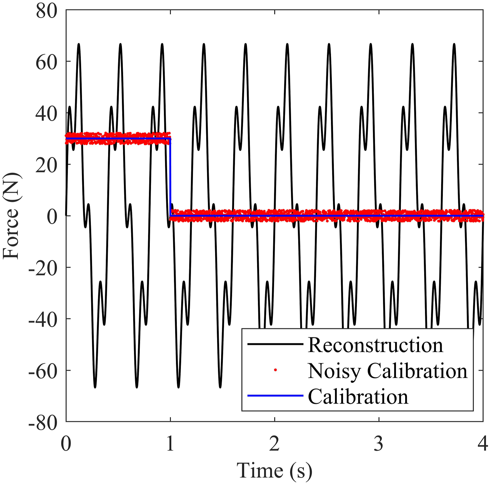
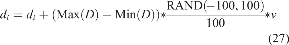
is the unit step function. The analytical solutions to the system with the applied forces described in equations (26a-b) were generated and used to verify the method.

f_{2} (t)

was used as the calibration case,

f_{C} (t)

f_{1} (t)

was used as the reconstruction case,

f_{R} (t)

. In fact, we also took the reversal and yielded similar behavior and accuracy findings. However, the step change is recommended as the preferred calibration by Frankel et al. (2017) owing to its inherent frequency decomposition characteristics. Seven percent (7%) random noise was added to these datasets, as illustrated in Figures 2 and 3, for simulating the acquired “measurement” data. The noise model used to add noise to a dataset

D = {d_{0}, \dots, d_{n}}

was

\begin{matrix} d_{i} = d_{i} + (Max (D) - Min (D)) * \frac{RAND (- 100, 100)}{100} * ν \end{matrix}

(27)

with

RAND (a, b)

defined as a random number between

a

and

b

, and

ν

as the specified noise level (7%). This model adds or subtracts up to

ν

percent of the range of

D

d_{i}

Figure 2.

Reconstruction and calibration forces.

Figure 3.

Reconstruction and calibration responses.

To numerically verify the method, data were generated at a sampling rate of 500 Hz for the two previously described forcing functions using analytically derived solutions for displacement. Figure 2 shows the defined forcing functions over time, $t \in [0,4] s$ . Figure 3 displays the time histories of the displacements for both cases with and without noise addition.

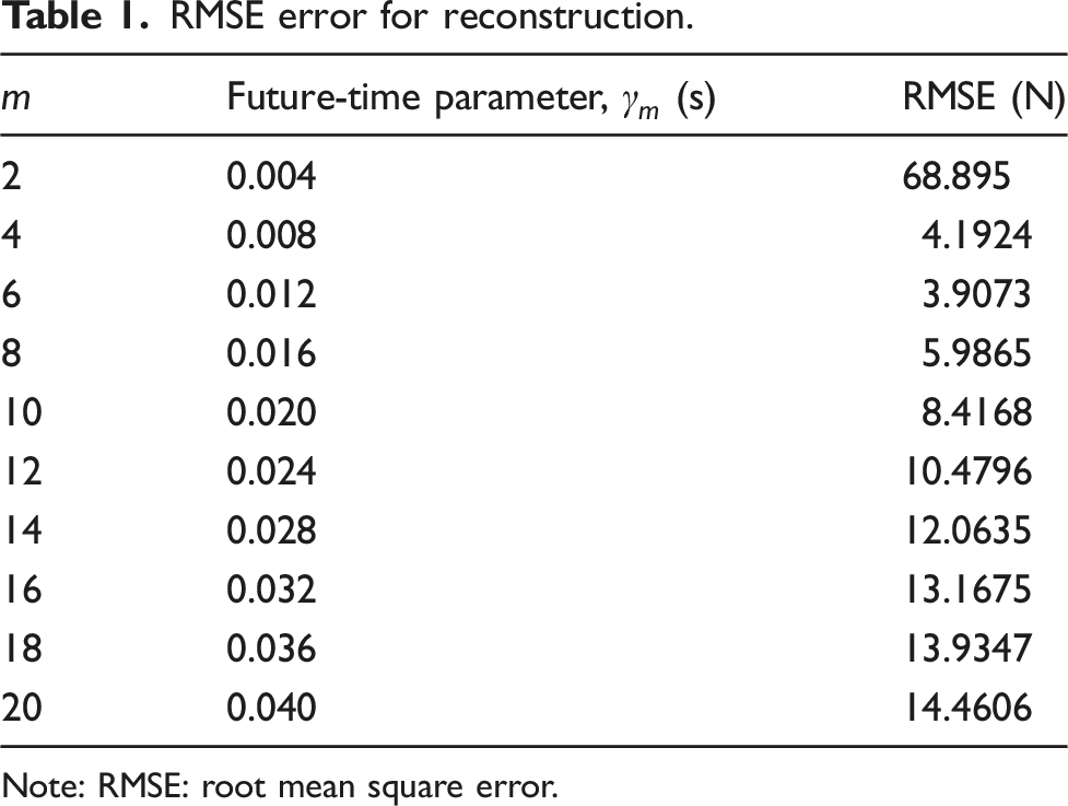
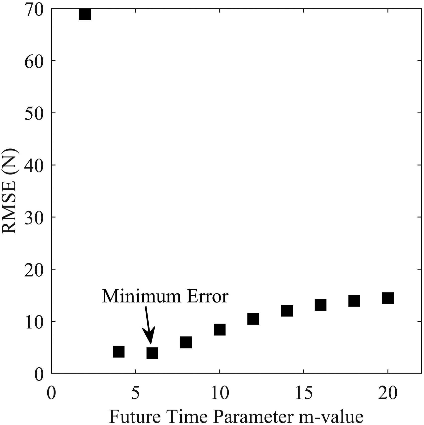
The optimal future-time parameter is chosen through the phase–plane and cross-correlation procedures described in Section 5. To do this, a family of forcing function predictions,

{\tilde{f}}_{R, γ_{m}, N} (t_{i}),

was assembled using 11 different future-time parameters, a first point to initialize cross correlation at

m = 1

, and iterating with

k = 1, \dots, P = 10

γ_{m} = k M_{f} Δ t, M_{f} = 2

, and

Δ t = 0.002 s

. After calculating the forcing function predictions for

{\tilde{f}}_{R, γ_{m}, N} (t_{i}), i = 0,1, \dots, N - k M_{f}

, over the

P + 1

future-time parameters, prediction sets

(m, m + 1)

were then cross correlated per the mathematical descriptions given in equations (23a-b). Figure 5 displays the results of this analysis using the phase–plane view. Table 1 presents the root mean square error (RMSE) of the reconstructed forcing function,

{\tilde{f}}_{R, γ_{m}, N} (t_{i}),

over the future-time parameters, while Figure 4 plots the RMSE of the reconstructed forcing function,

{\tilde{f}}_{R, γ_{m}, N} (t_{i}),

over the future-time index, m. From the following results, it is clear that

m = 6

γ_{6} = 0.012 s

produces the minimum error for this choice

M_{f}

. Normally, one plots two or three predictions about the estimated optimal regularization parameter.

Table 1.

RMSE error for reconstruction.

$m$	Future-time parameter, $γ_{m}$ (s)	RMSE (N)
2	0.004	68.895
4	0.008	4.1924
6	0.012	3.9073
8	0.016	5.9865
10	0.020	8.4168
12	0.024	10.4796
14	0.028	12.0635
16	0.032	13.1675
18	0.036	13.9347
20	0.040	14.4606

Note: RMSE: root mean square error.

Figure 4.

Root mean square error over Future Time Index, m.

The cross-correlation concept becomes important as the true error is not a calculable quantity in experimental situations. In Figure 5 and Table 2, there are a few distinct groups of cross-correlation coefficient pairings. The first noted group occurs near $ρ \in (0, 0.75)$ and $\dot{ρ} = 0$ . This group consisted of parameter index pairs $(m = 1, m = 2)$ and $(m = 2, m = 4)$ and it indicates instability that will be observed as large random predictions. A second grouping event occurs near $ρ = 1$ and $\dot{ρ} \to 1$ . In this case, the predictions become oversmoothed and damped with increasing future-time parameter. However, a region or “cusp” of stability is observed between these two extremes. Namely, from Figure 5, it is observed that the two future-time parameter sets $(m = 4, m = 6)$ and $(m = 6, m = 8)$ balancing the two extremes. From previous experimental and analytical studies (Frankel and Keyhani, 2017; Frankel et al., 2017) a representative value commonly used to guide occurs when setting the vertical cut-off near $\dot{ρ} = 0.75$ with this level of noise. From this, normally the “best” predictions will be based on using $m = 6$ or $m = 8$ .

Figure 5.

Cross-correlation phase plane.

Table 2.

Cross-correlation coefficients.

m-sets (m,m+1)	Future-time parameter, γ (s)	$ρ ({\tilde{f}}_{R, γ_{m}, N}, {\tilde{f}}_{R, γ_{m + 1}, N})$	$\dot{ρ} ({\dot{\tilde{f}}}_{R, γ_{m}, N}, {\dot{\tilde{f}}}_{R, γ_{m + 1}, N})$
1–2	(0.002, 0.004)	0.0038	−0.0027
2–4	(0.004, 0.008)	0.4947	0.0114
4–6	(0.008, 0.0012)	0.9951	0.5412
6–8	(0.0012, 0.016)	0.9962	0.6976
8–10	(0.016, 0.020)	0.9968	0.7698
10–12	(0.020, 0.024)	0.9977	0.8165
12–14	(0.024, 0.028)	0.9984	0.8534
14–16	(0.028, 0.032)	0.9989	0.8835
16–18	(0.032, 0.036)	0.9992	0.9067
18–20	(0.036, 0.040)	0.9994	0.9233

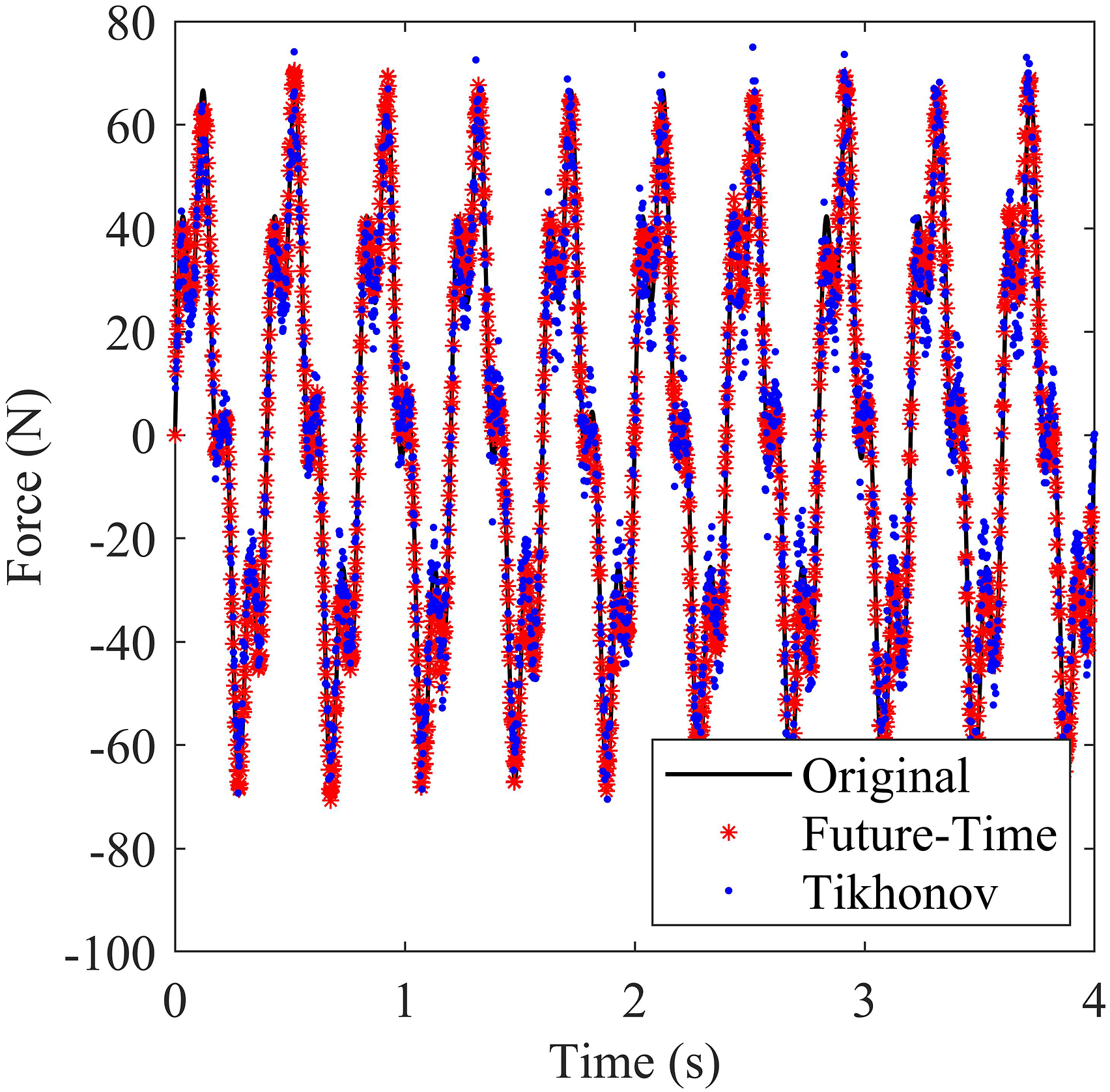
Figure 6 compares the exact forcing function, the future-time reconstruction based on $m = 6$ , and the Tikhonov regularization solution. This Tikhonov solution used a regularization parameter of $10^{- 8}$ which resulted in an $R M S E$ of $7.1884$ Newtons. It is observed that both future-time and Tikhonov regularization provide acceptable and accurate solutions to the problem at hand, and with adequate regularization parameters, there will be little or no differentiation between their solutions’ validity.

Figure 6.

Future-time optimal reconstruction.

An entire paper could be written comparing the future-time and Tikhonov approaches’ relative performance. Briefly, one advantage future-time regularization has is a more intuitive parameter selection process. Future-time parameter selection requires only iterating along integers. This contrasts sharply with the Tikhonov parameter selection, which required iterating on a log scale from $10^{- 11}$ to $10^{- 7}$ . An advantage of Tikhonov is the existing, optimized, open-source libraries containing ridge regression which can be easily pulled and used to implement Tikhonov regularization. Future-time’s current novelty removes it from the easy, “off the shelf” list of solutions. One last differentiator is the fact that future-time requires “sacrificing” a few data points at the end of the observation window. In the case of Figure 6, six of 2000 points were “sacrificed” to achieve the regularized solution. In many contexts, this fact will be inconsequential.

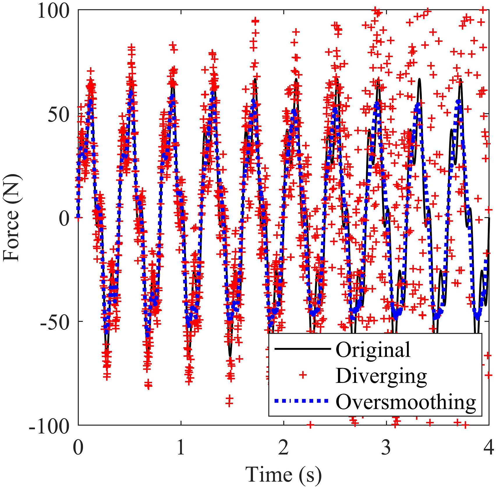
Figure 7 demonstrates the potential to regularize too much or too little and thus get a respectively unstable or oversmoothed solution. The diverging solution used $m = 2$ , which was expected to be unstable. This instability manifests as increasing magnitudes over time and random noise. The oversmoothed solution used $m = 14$ , and the solution loses features and magnitude over time. The Tikhonov approach has the same behavior when the solution is under or over regularized.

Figure 7.

Divergence and oversmoothing.

8. Conclusion

This article introduces a calibration framework for resolving the proposed inverse problem of any linear, time-invariant, initial-valued differential equation. Further, this view permits a reduction in systematic errors as no property input is required in this “parameter-free” formulation. The methodology suggested in this note is also applicable to “parameter required” inverse methods. In this case, the properties are specified, and no experimental calibration rig is required. Regularization is accomplished using a form of the future-time method. Cross-correlation and phase–plane principles are introduced for identifying the optimal prediction of the forcing function. Incorporation of these components produced a viable framework for resolving a calibration-reconstruction scheme. A numerical simulation was performed verifying the propositions described in this note. The proposed method solution was compared with the Tikhonov regularization method. Similar accuracy was observed between the two methods. This simulation solved the inverse problem of a MSD system, reconstruction the applied force from the response data.

Footnotes

Declaration of conflicting interests

The author(s) declared no potential conflicts of interest with respect to the research, authorship, and/or publication of this article.

Funding

The work reported here was supported by a grant provided to Dr. J.I. Frankel from the National Science Foundation (NSF-CBET-2031808). Mr. C. Rice received support from the Mechanical & Aerospace Engineering Departmental Scholarship through the University of Tennessee Department of Mechanical, Aerospace, and Biomedical Engineering.

ORCID iD

Chapel Rice

Appendix A

References

Beck

Blackwell

Clair

St.CR

Jr (1985) Inverse Heat Conduction. New York: Wiley.

Brownjohn

JMW

Bocian

Hester

, et al. (2016) Footbridge system identification using wireless inertial measurement units for force and response measurements. Journal of Sound and Vibrations 384: 339–355.

Chaigne

(2016) Reconstruction of piano hammer force from string velocity. The Journal of the Acoustical Society of America 140(5): 3504–3517.

Chen

Chan

THT

(2019a) Comparison of regularization methods for moving force identification with Ill-posed problems. Journal of Sound and Vibrations 478: 115349.

Chen

Qin

Zhao

, et al. (2019b) Toward efficacy of piecewise polynomial truncated singular value decomposition algorithm in moving force identification. Advances in Structural Engineering 22(12): 2687–2698.

Chen

Qin

Chan

THT

, et al. (2020) A novel preconditioned range restricted GMRES algorithm for moving force identification and its experimental validation. Mechanical Systems and Signal Processing 155: 107635.

Frankel

Chen

Keyhani

(2017) New step response formulation for inverse heat conduction. Journal of Thermophysics and Heat Transfer 31(4): 989–996.

Frankel

Keyhani

Elkins

(2013) Surface heat flux prediction through physics-based calibration, part 1: theory. Journal of Thermophysics and Heat Transfer 27(2): 189–205.

Frankel

Keyhani

(2017) Cross correlation and inverse heat conduction by a calibration method. Journal of Thermophysics and Heat Transfer 31(3): 746–756.

10.

Inoue

Harrigan

Reid

(2001) Review of inverse analysis for indirect measurement of impact force. Applied Mechanics Reviews 54: 503–524.

11.

Hwang

J-s

Kareem

Kim

W-j

(2009) Estimation of modal loads using structural response. Journal of Sound and Vibration 326: 522–539.

12.

Jacquelin

Bennani

Hamelin

(2003) Force reconstruction: analysis and regularization of a deconvolution problem. Journal of Sound and Vibration 265: 81–107.

13.

Jingjing

(2019) Identification of moving loads using a local linear embedding algorithm. Journal of Vibration and Control 25(11): 1780–1790.

14.

Kress

(1989) Linear Integral Equations. New York: Springer-Verlag.

15.

Linz

(1985) Analytical and Numerical Methods for Volterra Equations. Philadelphia: Society for Industrial and Applied Mathematics.

16.

Lamm

(2000) A survey of regularization methods for first-kind volterra equations. In: Engl

Louis

McLaughlin

, et al. (eds), Surveys on Solution Methods for Inverse Problems. New York: Springer Science and Business Media, 53–82.

17.

C-K

Chang

J-M

Lin

D-C

(2003) Input forces estimation of beam structures by an inverse method. Journal of Sound and Vibration 259: 387–407.

18.

Oppenheim

Schafer

(1975) Digital Signal Processing. Englewood Cliffs, NJ: Prentice-Hall.

19.

Qiau

Liu

, et al. (2019) An enhanced sparse regularization method for impact force identification. Mechanical Systems and Signal Processing 126: 341–367.

20.

Sneddon

(1995) Fourier Transforms. New York: Dover.

21.

Vogel

(1996) Non-convergence of the L-curve regularization parameter selection method. Inverse Problems 12: 535–547.

22.

Vyas

Wicks

(2001) Reconstruction of turbine blade forces from response data. Mechanism and Machine Theory 36: 177–188.

23.

Wing

(1991) Primer on Integral Equations of the First Kind. Philadelphia: Society for Industrial and Applied Mathematics.

24.

Woods

Lawrence

(1997) Modeling and Simulation of Dynamic Systems. New Jersey: Prentice-Hall.