Maximum likelihood estimation of the Markov chain model with macro data and the Ecological inference model

Abstract

This paper merges two isolated bodies of literature: the Markov chain model with macro data, formally described in detail by MacRae in 1977, and the Ecological inference model, the pitfalls of which were discussed by Robinson in 1950. Both are choice models. They have the same likelihood function and the same regression equation.

Decades ago, this likelihood function was computationally demanding. This has led to the use of several approximate methods, in particular with the Ecological inference model. Due to the improvement in computer hardware and software since Macrae (1977), the exact maximum likelihood should now be the preferred estimation method.

Keywords

Aggregated data macro data Markov chain Ecological inference computing time

1. Introduction

This paper merges two isolated bodies of literature: respectively about the first order Markov chain model with macro data and about the Ecological inference model. They contain very few references to each other, while in fact they are equivalent in the sense that they have the same likelihood function and the same regression equation.

Moreover, this paper disproves the general opinion that the computational burden of this likelihood function is still so large that one should rather use an approximation, or a subsample of the data.

In Sections 2 and 3, the two models are described with their respective typical examples, followed by a common notation in Section 4. In Sections 5 and 6 the likelihood function and the regression equation are given.

In Section 7 a numerical example is given, followed by the conclusions in Section 8.

All discussions below are limited to binary classifications. This is sufficient for the purpose. In fact, most of the Ecological literature is (double) binary.

2. The Markov chain model with macro data

A Markov chain model is a time series model for panels with discrete data. We consider the first-order model, with lags of only one time period.

In the binary case, at each time period the individuals in the panel are in one of two states. For instance, employed or unemployed: the probability for an individual to be employed in a given time period depends on being employed or not in the previous time period.

With the original micro panel data, these probabilities can be estimated easily, based on (for each time period except the first) the cross tabulation of the state in that time period against the state in the previous time period. With aggregated panel data this tabulation is not available; only the marginal frequencies are available and estimation of the probabilities is harder.

A short review of the subject’s history over the past four decades is as follows. [1, 2] are forerunners, discussing mainly regression analysis. They also discuss an approximate likelihood function where the data are assumed to be multinomially distributed (which they are not). In the seminal [3], regression analysis and exact maximum likelihood are compared. She concludes:

While it is possible to develop computational algorithms to search for a maximum [likelihood], the iterative generalized least squares estimator may represent a better combination of numerical and statistical efficiency.

In [4] the combined use of micro and macro data is discussed, with a large list of references. In [5] the history of theoretical and applied work on the subject is reviewed (though not including [3]) with the conclusion that the computation of the exact likelihood function is “unfeasible” (p. 3202).

3. The Ecological inference model

Here, the word “Ecological” (capitalized) has little to do with subjects like pollution, growing crops without chemicals, etcetera. Rather, as the title of [6] indicates, it is about “reconstructing individual behavior from aggregate data”; compare with the title of [3].

Hence, by definition in an Ecological inference model the data are aggregated. Time usually does not play a role and instead of time periods we usually have regions. In the 2 $\times$ 2 case we have two dichotomies, with data for each region. One of the two dichotomies plays the role of the lagged information in the Markov chain model; this dichotomy might refer to a property of individuals which is constant over their life.

The standard example of this dichotomy is race, where the other dichotomy is political preference: the probability of having a given political preference depends on one’s race. The data consist of the two marginal frequency distributions, concerning race and political preference respectively, for multiple regions. Naturally, where political preferences are expressed by some secret ballot, the results are only available in this form.

The seminal paper is [7]. In [8] the background and the state of the research at the time is discussed. It is noted that the exact likelihood “has rarely been explicitly considered in the Ecological inference literature” (top of p. 391). See also the introductory chapter in [9]. To the best of my knowledge, the authors of [10] were the first to apply the exact likelihood, though only to a small part of their data.

4. A common notation

4.1 The Markov chain model

In the Markov chain model, we have ${I}+1$ observations over time. This gives a chain of ${I}$ transitions from one time period to the next. Referring to the employment example above, the $x_{{i}}$ are the first ${I}$ frequencies of employed individuals and the $y_{{i}}$ are the last ${I}$ frequencies, giving

$\displaystyle x_{{i}}=y_{{i}-1}$ (1)

Note that we have no initial conditions problem here, such as in a time series regression model with a lagged error term.

The symbol $p_{1{i}}$ is the probability that an individual included in the number $x_{{i}}$ is also included in the number $y_{{i}}$ . Likewise, $p_{2{i}}$ is the probability that an individual not included in the number $x_{{i}}$ is included in the number $y_{{i}}$ . Below I will use “unit” as the general term for the ${i}$ index.

Ignoring panel attrition, the $n_{i}$ series in the Markov chain model is constant over ${i}$ , say $n_{i}=n$ . With also constant probabilities $p_{1}$ and $p_{2}$ , the fraction $y_{{i}}/n$ moves, with random ups and downs, in the direction of $P=p_{2}/(1-p_{1}+p_{2})$ , the solution of $p_{1}P+p_{2}(1-P)=P$ .

4.2 The Ecological inference model

Here, typically the units are regions, without inherent ordering, indexed by ${i}=1,\dots,{I}$ . Unit ${i}$ has $n_{i}$ individuals. Using the above standard example in the Ecological model, $y_{{i}}$ is the number of individuals in unit ${i}$ who have the reference political preference and $x_{{i}}$ is the number of individuals with the reference race.

Hence $p_{1{i}}$ is the probability that an individual in unit ${i}$ with the reference race has the reference political preference and $p_{2{i}}$ is the probability that an individual in ${i}$ , not with the reference race, has the reference political preference.

4.3 The relations between the frequencies

Table 1 shows the frequencies. Since the data are aggregated, only the totals are observed; the remaining four numbers are not observed. However, if any one of these four numbers would be known then the other three would also be known. Without loss of generality I choose $k_{{i}}$ as the index of all possible sets of four unobserved frequencies, given the observed totals.

Table 1
The frequencies in unit ${i}$ , with the index frequency $k_{{i}}$

Lagged (Markov chain)	Unlagged (Markov chain)
or race (typical Ecological)	or political preference (typical Ecological)
	In reference state	Else	Total
In reference state	$k_{{i}}$	$x_{{i}}-k_{{i}}$	$x_{{i}}$
Else	$y_{{i}}-k_{{i}}$	$n_{i}-x_{{i}}-y_{{i}}+k_{{i}}$	$n_{i}-x_{{i}}$
Total	$y_{{i}}$	$n_{i}-y_{{i}}$	$n_{i}$

Notes. Only totals are observed. The word “state” does not refer to the states of the United States.

4.4 Exogenous variables

The probabilities may depend on macro exogenous variables as follows. For all ${i}$ :

$\displaystyle p_{1{i}}=F(\bm{z}_{{i}1}\bm{\beta}_{1})\text{ and }p_{2{i}}=F(% \bm{z}_{{i}2}\bm{\beta}_{2})$ (2)

where the $\bm{z}_{{i}1}$ and $\bm{z}_{{i}2}$ are rows from exogenous data matrices $\bm{Z}_{1}$ and $\bm{Z}_{2}$ , respectively (These two matrices may have columns in common.). The $\bm{\beta}_{1}$ and $\bm{\beta}_{2}$ are unknown column vectors of parameters (They may have elements in common.).

The function $F$ is a strictly monotonous transformation from the real line to the zero-one range, such as the logit and probit functions. See [3], p. 185. In order to obviate the use of inequality restrictions on the parameters, one might use such a function even without exogenous variables, with $p_{1}=F(\bm{\beta}_{1})$ and $p_{2}=F(\bm{\beta}_{2})$ and scalar $\bm{\beta}_{1}$ and $\bm{\beta}_{2}$ . This is done in the example below, with $F$ being the logit function.

5. The likelihood function

The unconditional distribution of $k_{{i}}$ and of $y_{{i}}-k_{{i}}$ ; i.e., not considering $y_{{i}}$ as given, is:1

$\displaystyle\mathrm{Pr}\left(k_{{i}}|x_{{i}},\bm{\beta}_{1}\right)=\mathrm{B}% (k_{{i}},x_{{i}},p_{1{i}})$ $\displaystyle\mathrm{Pr}\left(y_{{i}}-k_{{i}}|x_{{i}},\bm{\beta}_{2}\right)=% \mathrm{B}(y_{{i}}-k_{{i}},n_{i}-x_{{i}},p_{2{i}})$ (3)

taking into account Eq. (2). The B indicates the binomial probability with $\mathrm{B}(k,n,p)=\binom{n}{k}p^{k}(1-p)^{n-k}$ .

The $y_{{i}}$ are distributed as follows:

$\displaystyle\mathrm{Pr}\left(y_{{i}}|x_{{i}},\bm{\beta}_{1},\bm{\beta}_{2}% \right)=\sum_{k_{{i}}}\mathrm{Pr}\left(k_{{i}}|x_{{i}},\bm{\beta}_{1}\right)% \mathrm{Pr}\left(y_{{i}}-k_{{i}}|x_{{i}},\bm{\beta}_{2}\right)$ (4)

where the range of the summation is

$\displaystyle\max(0,x_{{i}}+y_{{i}}-n_{i})\leqslant k_{{i}}\leqslant\min(x_{{i% }},y_{{i}})$ (5)

The likelihood function is:

$\displaystyle L\left(\bm{\beta}_{1},\bm{\beta}_{2}\right)=\prod_{{i}=1}^{I}% \mathrm{Pr}\left(y_{{i}}|x_{{i}},\bm{\beta}_{1},\bm{\beta}_{2}\right)$ (6)

For the first order Markov chain model, see [3], with the general case, not limited to binary choice. For the Ecological model, see for instance [8]Eq. (4), discussed at the top of page 391 (as noted above) and [11] Eq. (1.6). In [10] the first order derivatives of the loglikelihood and the Fisher information matrix are given, with a numerical application.

This likelihood is computationally more demanding than ordinary binary choice models: the computing time of Eq. (6) is roughly equal to the computing time of an ordinary binary choice model, times the sum over the units ${i}$ of the size of the range of $k_{{i}}$ in Eq. (5). Of course, this sum might be anything from a few hundred to, say, a few hundred thousand.

In order to distinguish between this likelihood and its approximations,2 in the binary case this likelihood is often called the convolution likelihood, named after the convolution sum in discrete form in the right-hand side of Eq. (4).

6. Least squares regression

With Eq. (5) we have:

$\displaystyle\mathrm{E}\left[y_{{i}}|x_{{i}},\bm{\beta}_{1},\bm{\beta}_{2}% \right]=\mathrm{E}\left[k_{{i}}|x_{{i}},\bm{\beta}_{1}\right]+\mathrm{E}\left[% y_{{i}}-k_{{i}}|x_{{i}},\bm{\beta}_{2}\right]=x_{{i}}p_{1{i}}+\left(n_{i}-x_{{% i}}\right)p_{2{i}}$ (7)

With constant $p_{1}$ and $p_{2}$ we have for all ${i}$ :

$\displaystyle\frac{\mathrm{d}\,\mathrm{E}\left[y_{{i}}|x_{{i}},\bm{\beta}_{1},% \bm{\beta}_{2}\right]}{\mathrm{d}\,x_{{i}}}=p_{1}-p_{2}$ (8)

In words: the difference between the two probabilities is a reflection of the correlation over the regions between $x_{{i}}$ and $y_{{i}}$ .

Equation (7) is a regression equation with the following error variance:

$\displaystyle\mathrm{V}\left[y_{{i}}|x_{{i}},\bm{\beta}_{1},\bm{\beta}_{2}% \right]=x_{{i}}p_{1{i}}\left(1-p_{1{i}}\right)+\left(n_{i}-x_{{i}}\right)p_{2{% i}}\left(1-p_{2{i}}\right)$ (9)

Hence Eq. (7) can be estimated with nonlinear Feasible Generalized Least Squares (FGLS) by minimizing

$\displaystyle\sum_{{i}}\frac{\left(y_{{i}}-\mathrm{E}[y_{{i}}|x_{{i}},\bm{% \beta}_{1},\bm{\beta}_{2}]\right)^{2}}{\mathrm{V}\left[y_{{i}}|x_{{i}},\bm{% \beta}_{1},\bm{\beta}_{2}\right]}$ (10)

See [3, p. 189/190].

Unlike the maximum likelihood estimate, this regression estimate is independent of the sample size, in the following sense. Replacing all $y_{{i}}$ and all $x_{{i}}$ and all $n_{i}$ by their multiplication with a nonzero scalar, say $m$ , gives for the minimand Eq. (10):

$\displaystyle\sum_{{i}}\frac{\left(my_{{i}}-m\mathrm{E}[\dots]\right)^{2}}{m% \mathrm{V}\left[\dots\right]}=m\sum_{{i}}\frac{\left(y_{{i}}-\mathrm{E}[\dots]% \right)^{2}}{\mathrm{V}\left[\dots\right]}$ (11)

This expression has its minumum at the same parameter values as Eq. (10). This is illustrated in Section 7; with increasing sample size, the maximum likelihood estimate converges to the constant least squares estimate.3

7. Example

Table 2
Percentage employment among women

Year	%	Year	%
1986	40.0	1991	47.6
1987	40.6	1992	51.5
1988	42.5	1993	52.5
1989	43.2	1994	52.6
1990	44.8	1995	55.7

Source: [12].

In order to study computing times and to illustrate some other issues, I computed the exact likelihood, with a Markov chain model, using the times series data of [12]. Although that paper is not about panels, the data come from a panel. The panel contains women who are either employed or unemployed. The percentages are in Table 2. The first nine percentages are the $x_{{i}}/n_{i}$ series and the last nine are the $y_{{i}}/n_{i}$ series. The sample size $n_{i}$ (not shown here) changes somewhat over time, with an average of 2200 persons. No exogenous variables are used.

Table 3

Estimates of probabilities for the Pelzer data

	$n_{i}=n$	$1-p_{1}$	$p_{2}$	Long run $y_{{i}}/n=$
				$p_{2}/(1-p_{1}+p_{2})$
		%
Maximum likelihood	220	1.6	4.6	75
	2200	8.5	10.5	55
	22000	9.8	11.7	54
FGLS regression	any	10	12	54

Note: when employed: $p_{1}=$ Pr (keeping employment); when unemployed: $p_{2}=$ Pr (finding employment).

The estimates are in Table 3, with simulated sample sizes. As discussed above: unlike the maximum likelihood estimate, the least squares estimate does not change with the sample size.4 The difference between the two decreases with increasing sample size.

Figure 1 shows a contour map of the loglikelihood over the ( $p_{1},p_{2}$ ) unit square, with $n_{i}=n=220$ . This differs most from the least squares regression (FGLS). The map strongly suggests that here we have a global and well defined maximum.

Figure 1.

Contour plot of the log likelihood for 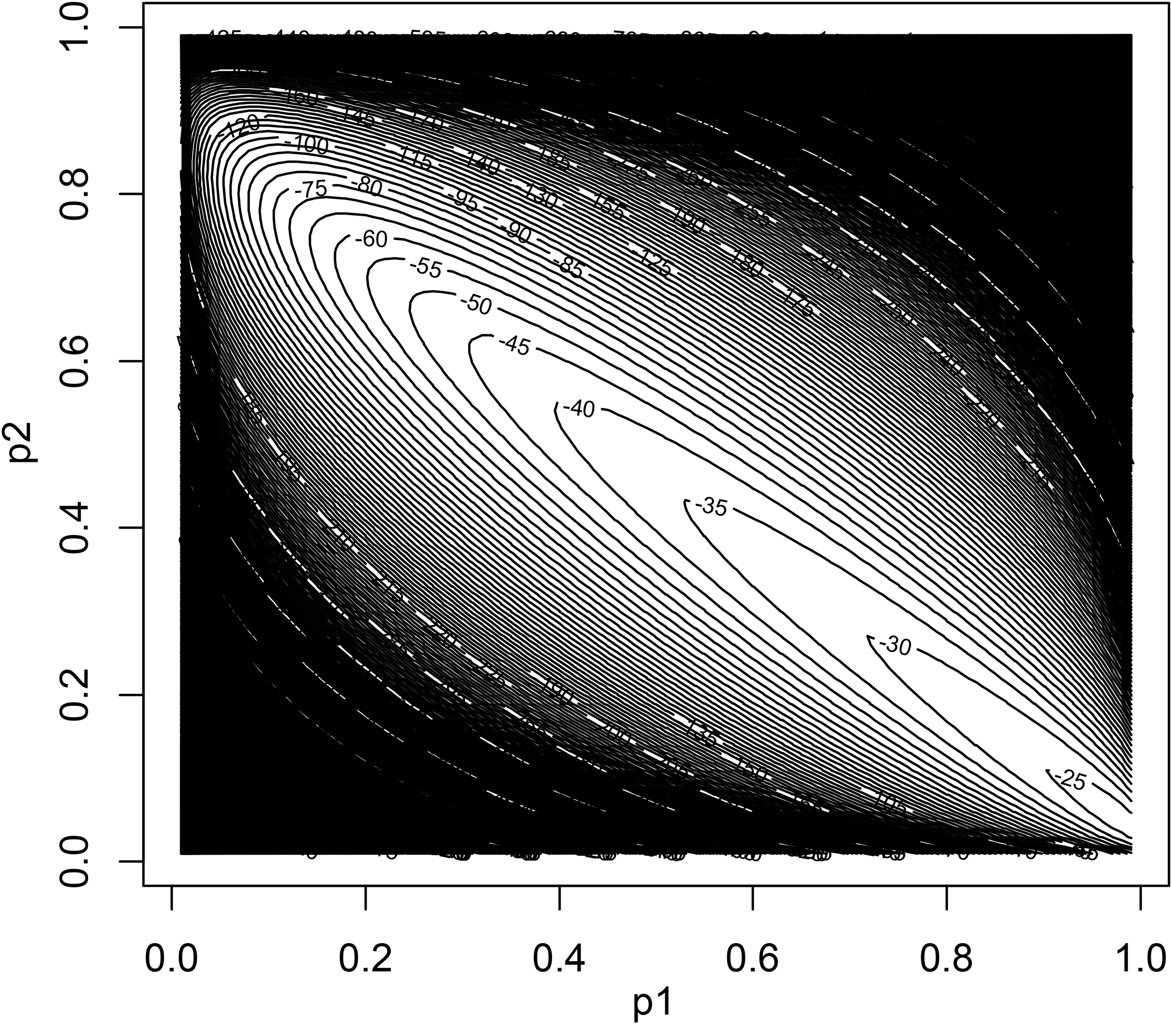$n_{i}=n=220$ .

I saw no need to use here the EM algorithm, which is slower (though more robust) than the Newton algorithm. See [13], Section 3.2 for the EM algorithm applied to this likelihood function.

For the largest sample size (22000), the computing time (without a contour plot) was slightly under ten seconds on a laptop PC with an 1.7 GHz Intel processor and 4 GB RAM. I used the built-in array facilities of the R language (version 3.0.0, Windows 8, 64 bits) with the nlm function.

8. Conclusions

The first order Markov chain model with macro data can be considered as a special case of the Ecological inference model, with the two classifications of the Ecological model being the same, recorded at two subsequent time periods. Students of this Markov model might consult [10] for details of the exact likelihood function, which can be translated to the Markov model using the current paper.

Students of Ecological inference might have benefited from reading [3] at that time. Both might do well no longer to dismiss out of hand the exact likelihood as unfeasible.

The maximum likelihood estimate differs most from the least squares regression in small samples, where the computation of the likelihood function is less of a problem.

Remaining work: find out more about the possibility of multiple likelihood maxima. Note: in the case of one unit ( $I=$ 1), the loglikelihood is saddle shaped, with multiple border maxima; see for instance Figs 1.6(a) and 1.8(a) of [11].

Footnotes

For brevity I write for example $\mathrm{Pr}({x})=\phi(x)$ , instead of the more precise $\mathrm{Pr}(x=X)=\phi(X)$ .

A quite different distribution of $k_{{i}}$ and $y_{{i}}-k_{{i}}$ (given $x_{{i}}$ ) is presented in [6], pp. 93/94: the fractions $k_{{i}}/x_{{i}}$ and $(y_{{i}}-k_{{i}})/(n_{i}-x_{{i}})$ are drawn from a truncated bivariate normal distribution. Compare the first line of the first formula on his page 308 with our Eq. (4). This model has been adapted and refined; see [], Section 0.1.4.

Loosely speaking this convergence follows from: (a) with increasing $n$ , a binomial mass distribution converges to a normal density distribution and (b) the convolution integral of two normal density distributions is again a normal density distribution and (c) with normally distributed $y$ , least squares gives the same result as maximum likelihood. See also for instance [, p. 20/21].

In fact, there is some “random” noise in the regression estimates, due to the rounding of the frequencies computed from the percentages in Table . Hence the rounding of the 10 and the 12 in the bottom line of the table; the first digit after the decimal comma varies somewhat among the sample sizes.

Acknowledgments

The author thanks Stefan Boeters and Sander Muns and Marno Verbeek for their comments on earlier versions and Gary King for his willingness to reply to my questions about his book and his data.

Supplementary data

The supplementary files are available to download from http://dx.doi.org/10.3233/ JEM-452.

References

Lee

Judge

Zellner

. Estimating the Parameters of the Markov Probability Model From Aggregate Time Series Data. North Holland; 1970.

Dent

Ballintine

. A review of the estimation of transition probabilities in Markov chains. The Australian Journal of Agricultural Economics. 1971; 15: 69–81.

MacRae

. Estimation of Time-Varying Markov Processes with Aggregate Data. Econometrica. 1977; 45: 183–198.

Rosenqvist

. Micro and Macro Data in Statistical Inference on Markov Chains. Publications of the Swedish School of Economics and Business Administration, nr 36; 1986.

Crowder

Stephens

. On inference from Markov chain macro-data using transforms. Journal of Statistical Planning and Inference. 2011; 141: 3201–3216.

King

. A Solution to the Ecological Inference Problem: Reconstructing Individual Behavior from Aggregate Data. Princeton University Press; 1997.

Robinson

. Ecological Correlations and the Behavior of Individuals. American Sociological Review. 1950; 15: 351–357.

Wakefield

. Ecological inference for 2 × 2 tables. Journal of the Royal Statistical Society, Series A. 2004; 167(Part 3): 385–445.

King

Rosen

Tanner

, eds. Ecological Inference: New Methodological Strategies. 1st ed. Cambridge University Press; 2004.

10.

Steel

Beh

Chambers

. The Information in Aggregate Data. In: King

Rosen

Tanner

, eds. Ecological Inference: New Methodological Strategies. 1st ed. Cambridge University Press; 2004. p. 51–68.

11.

Wakefield

. Prior and Likelihood Choices in the Analysis of Ecological Data. In: King

Rosen

Tanner

, eds. Ecological Inference: New Methodological Strategies. 1st ed. Cambridge University Press; 2004. p. 13–50.

12.

Pelzer

Eisinga

Franses

. Estimating transition probabilities from a time series of independent cross sections. Statistica Neerlandica. 2001; 55: 249–262.

13.

Eisinga

. Information loss for 2 × 2 tables with missing cell counts: binomial case. Statistica Neerlandica. 2008; 62: 239–254.

Maximum likelihood estimation of the Markov chain model with macro data and the Ecological inference model

Abstract

Keywords

1. Introduction

2. The Markov chain model with macro data

3. The Ecological inference model

4. A common notation

4.1 The Markov chain model

4.3 The relations between the frequencies

Table 1 The frequencies in unit i , with the index frequency k i

Table 2 Percentage employment among women

Footnotes

Acknowledgments

Supplementary data

References

Table 1
The frequencies in unit ${i}$ , with the index frequency $k_{{i}}$

Table 2
Percentage employment among women