






Abstract
The objective in using the Kelly criterion for money management is to maximize returns; however, in many cases, the risk level exceeds that which the investor can bear. In this study, we present an algorithm to calculate the bidding fraction, while taking into account the level of risk (i.e., the maximum drawdown). The proposed algorithm is based on ensemble learning with a combination of bagging and subset resampling. Our assessment results obtained using the FF48 (i.e., Fama-French-48) dataset revealed that when the maximum drawdown was 5% and 10%, ensemble learning outperformed the conventional approach by 2% and 4%, respectively.
Introduction
Since its introduction in 1956 [1], the Kelly criterion has been one of the most popular approaches to asset allocation. This principle provides systematic guidance to maximizing the long-term growth rate of wealth in repeated gambling scenarios. It has also inspired the development of the growth-optimum portfolio [3].
The Kelly criterion refers to the fraction of assets that should be put at risk throughout the investment period in order to maximize wealth over the long term (i.e. with infinite bets). Unfortunately, the Kelly criterion disregards potential drawdown to the portfolio. In this study, we developed a systematic methodology by which to determine the most suitable fraction of assets to invest when the maximum drawdown is taken into account.
In a typical Kelly criterion problem, any given game can have only two outcomes: win (with probability of p) or lose (with probability of 1 - p). The formulation of the two outcomes is as follows: We earn b1 dollars or lose b2 for each dollar included in a bet. Thus, the optimal fraction (f*) of the Kelly formula can be derived as Equation (1).
This result implies that if we bet fraction f* of our available assets in each period, then our wealth can be maximized over the long term (assuming that the probability of winning is p). However, pundits of the Kelly criterion point out that this ignores the amount of risk that the investor is willing able to assume. In other words, the fraction derived using the Kelly criterion would be the same for any investor, regardless of their risk tolerance.
Before an investor obtains a return from an investment, there is always a risk of subsequent losses. Most conventional methods based on the Kelly criterion do not address this issue, and those that do generally impose a tradeoff between risk and returns. A popular variation is referred to as fractional Kelly [5, 6]; however, that approach has many detractors [8].
Our objective in this study was to resolve the shortcomings of the conventional Kelly criterion by taking the maximum drawdown into account. We developed a mathematical approach to deriving the bounds of drawdown probability in a classical Kelly gambling problem. We have revised the definition of drawdown as Equation (2).
In the current study, maximum drawdown was simulated using the method described in [7]. Monte Carlo simulation is used to derive the results for single asset problems, whereas ensemble learning is used to derive results for multiple asset problems.
Advances in communication [19, 20] and authentication technology [21, 22] have greatly increased the amount of available information. Numerous data mining methods have been developed to deal with this expanding body of knowledge [24]. Nonetheless, it is remains difficult for portfolio managers to determine the most suitable fraction. Thus, we also developed an ensemble-learning method to determine the optimal weighting scheme for the construction of a portfolio.
Ensemble learning has been implemented in machine learning schemes (mostly using bootstrapping); however, it is not easily applied in the field of portfolio management. One well-known problem involves the stationarity of model parameters [13], wherein the first two moments of returns do not remain constant throughout the entire time-series dataset. The statistical problem can be resolved using additional data from the same period; however, the availability of such historical data tends to be limited. In [14], the authors proposed a method by which to resample data to overcome this problem; however, other researchers [15] have pointed out that this approach seldom outperforms the Markowitz mean-variance portfolio.
The method described in [14] could be considered ensemble learning based on the bootstrap aggregating algorithm (i.e., Bagging). The method described in [16] uses the random subspace method or subset sampling to improve on the basic model. Intuitively, when using a complete dataset (rather than a subspace) as a sampling pool, the learner is susceptible to highly predictive features appearing in the training data, which tends to compromise performance when the learner is applied to an out-of-sample dataset [17]. Random subspace sampling is meant to prevent weak learners from being overly affected by such features. The results in [18] demonstrate the effectiveness of ensemble learning in conjunction with random subspace sampling. In the current study, we adopted the ensemble learning approach described in [18] to identify the most suitable fraction of assets invested for a given maximum acceptable drawdown.
When applying the Kelly criterion to problems involving a single asset, we used Monte Carlo simulation to reveal the relationship between the most suitable fraction of assets invested and the maximum acceptable drawdown. When considering multiple assets (i.e., determining the optimal weight for a portfolio), we use ensemble learning in conjunction with subset resampling to overcome the difficulties in dealing with out-of-sample data. When applied to a problem involving multiple assets, the proposed ensemble learning scheme was shown to outperform conventional methods in terms of overall returns and the degree of risk assumed by the investor.
Definition of risk for investors
In the traditional Kelly gambling problem, a player can put money into only one underlying random variable; however, an investor in the generalized version bets on more than one item at a time. Thus, we defined a vector to describe the strategy used to determine the bidding fraction as Equation (4).
The
Nonetheless, the definition of Wmin is not necessarily practical for all scenarios. Many investors are concerned about drawdown after reaching peak wealth. Thus, we use MDD (maximum drawdown) rather than the Wmin as the measurement of risk defined in Equation (7).
Then, Equation (5) can be reformulated as Equation (8).
This study sought to capture risk throughout the entire investment period using the algorithm described below. We first use α to define the upper bound of the maximum drawdown and β to define the probability of capping the maximum drawdown for a given α. Both metrics can be simplified using the Equation (2). i.e.
We first had to determine whether the most suitable fraction of assets invested could be determined when using set values for α and β. We then had to determine whether the most suitable fraction of assets invested could be used to reduce the risks faced by the investor without sacrificing the desired return. Note that we were constrained in calculating the most suitable fraction of assets to invest by the values selected for α and β as well as the need to maximize the expected wealth of the investor. Briefly, we designed a Monte Carlo-type algorithm based on the arguments listed in Table 1. Using Equation (8) to identify the most suitable fraction made it possible to account for the long-term returns as well as the degree of risk that the investor would be able to bear.
Parameters for single asset Algorithm
Parameters for single asset Algorithm
Optimizing a portfolio is more complex than dealing with a single asset.
We are interested only in the most recent data; therefore, in Equation (9), the objective function sums up only the values from period k - τ + 1 to period k, where τ indicates the window length and R
l
indicates the gross return vector at time l. In addition to the original constraint (
The objective function and desired MDD level can then be used to construct an algorithm to evaluate the relationship between portfolio returns and the corresponding probability.
We also designed an algorithm based on ensemble learning to calculate the optimal weight for a given portfolio, where the MDD of the portfolio is used as one of the arguments.
Monte Carlo method
As mentioned in the previous section, the proposed algorithm for a single asset is based on the Monte Carlo method. Once the number of experiments is specified, it is should be possible to determine the length of each experiment (i.e., the number of bets a player can make – number of iterations). The algorithm begins by simulating a player entering a casino n times, and betting several times during each stay. Note that Algorithm 1 samples a return ratio rather than absolute wealth. Table 2 describes an example experiment sequence.
Simulation example
Simulation example
In Algorithm 1, we first execute 2 layers as loops (Lines 4 and 5). The outer loop (Line 4) is executed n times (where i = 1 ∼ n), indicating a sweep from the first experiment to the nth experiment. Next, the inner loop (Line 5) increases f from 0.05 to 1 in increments of 0.05. This is the means by which the MDD of each of the n experiments is derived with various fractions of assets invested.
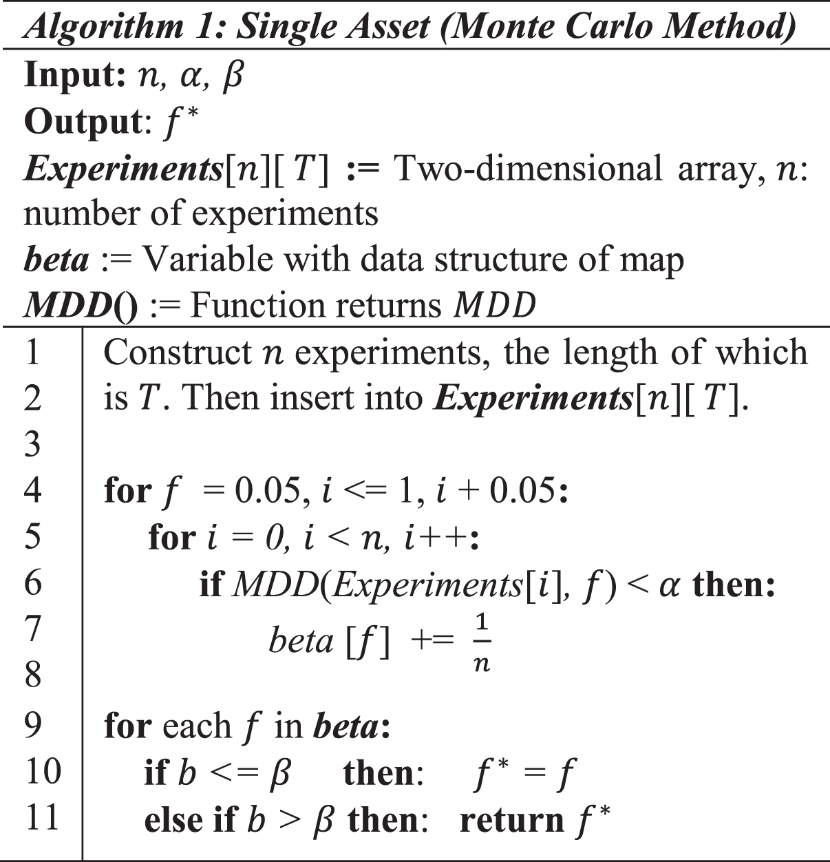
In Line 6, all of the MDD values are checked. If an MDD value is less than α, then it is recorded by Line 7. However, only the probability of success is recorded, such that beta [f] increases by
This algorithm uses the values α and β (specified by the investor) to calculate the most suitable fraction of assets to invest based on the desired degree of risk.
The following algorithm is a variation of the scheme presented in [9]. The outer loop (line 1) and inner loop (line 4) respectively refer to bagging and subset resampling. The four parameters (n1, n2, n3, and n4) can be tuned to adjust the outcome. In this study, we focused on the ensemble growth optimal (EGO) model with the four parameters respectively configured as 50, 60, 60, and n0.5.
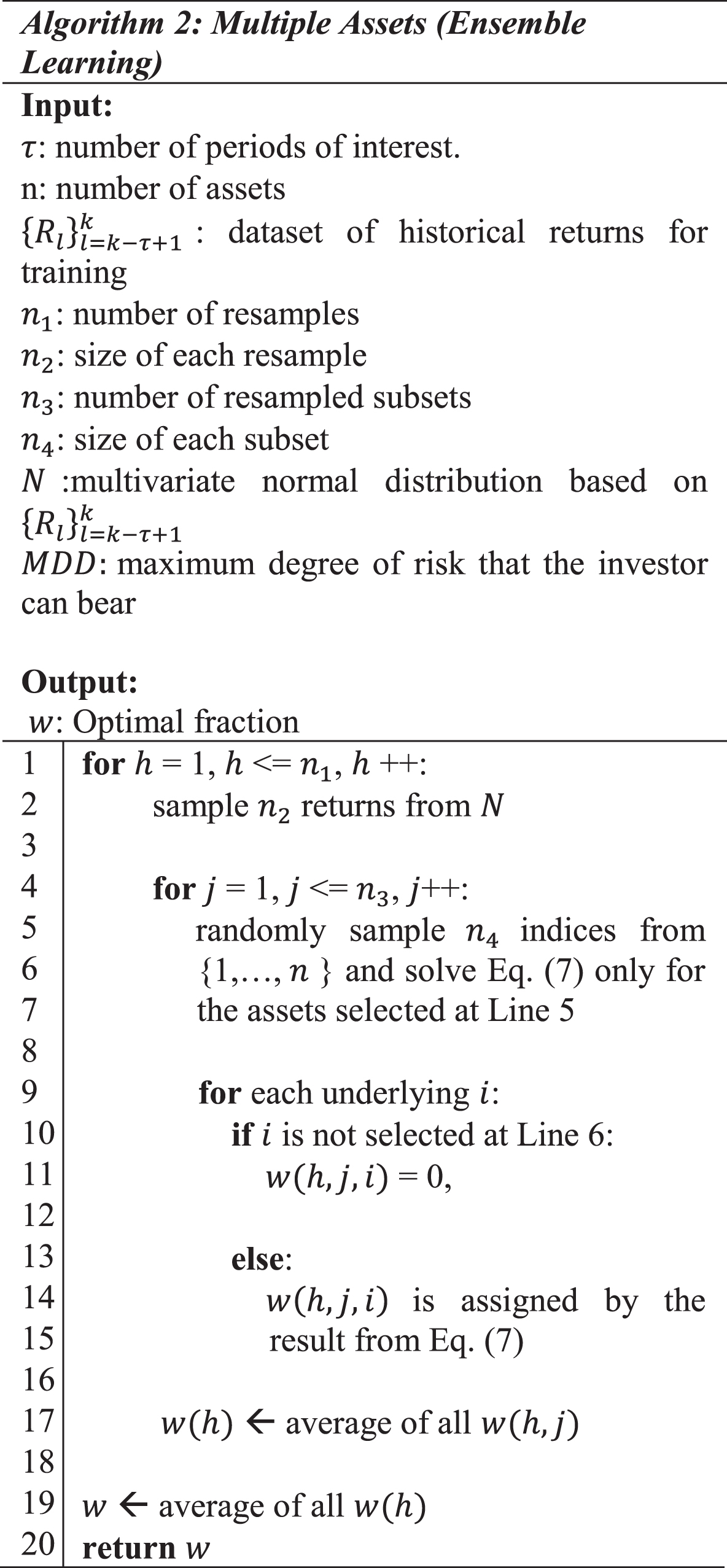
As mentioned in the previous section, ensemble learning is used primarily to leverage the power of subset sampling. Thus, when Algorithm 2 solves Equation (7) (Lines 5 – 7), only the chosen assets are considered. This means that there is no need to employ all of the underlying parameters as arguments to derive the optimal weight. The goal of subset sampling is to improve performance when dealing with out-of-sample data. Intuitively, when using an entire dataset (rather than a subspace) as a sampling pool, the learner should be affected by highly predictive features appearing in the training data, which could result in poor performance when out-of-sample data are encountered. Random subspace sampling can prevent weak learners from focusing too heavily on such features.
If the underlying parameter comprises only a single asset, then the algorithm degenerates to single asset conditions. Furthermore, if n4 equals n, then the effect of subset sampling disappears, due to the fact that subset sampling has meaning only when n4 is less than n. The conventional approach is defined with n4 equaling n (i.e., subset sampling is not adopted). The conventional approach is used each time the inner loop (Line 4) is executed, unless n4 is less than n, in which case subset sampling is used.
Note that if the underlying parameter is only a single asset, then the algorithm degenerates to a single asset. Note also that if n4 is equal to n, then the effect of subset sampling is nullified. This approach using subset sampling (inner loop) outperforms the conventional approach (i.e., n4 = n). Details related to this performance are provided in the following section.
Simulations and experiments
Simulation of single asset using algorithm based on Monte Carlo method
In the following, we use a simple coin toss to introduce the concept of risk within a game. The binary nature of a coin toss outcome is analogous to using a single asset. As described in the previous section, Algorithm 1 plays an important role in identifying the most suitable fraction of assets to invest. In the first two scenarios, α and the fraction of assets that should be put at risk are assigned specific values in order to illustrate the effects on returns and risk. Note that MDD is used as a metric in assessing risk.
In Fig. 1, α is fixed at 30%, which means that the investor cannot afford a portfolio loss exceeding 30% of its total value. The odds of the possible outcomes are 2 and -1, which means that if an investor gambled $1 on each bet, then he/ she would earn $1 or lose $1 in each round with a probability of 50%.
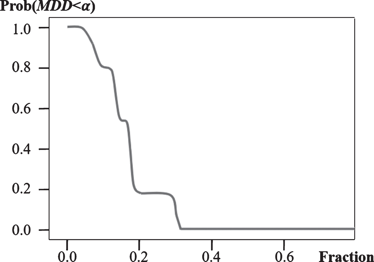
Simulation of single asset with α fixed at 30% and probability of winning fixed at 50% (i.e., odds of 2 and -1).
As shown in Fig. 1, the probability of MDD dropping below 30% decreases with the increment of the fraction of assets put at risk. When the fraction of assets at risk exceeds 30%, β is close to zero. In the example in Fig. 1, the fraction of assets risked on any given bet should not exceed 10% in order to avoid losing more than 30% of the total assets.
The situation in Fig. 2 has the bidding fraction fixed at 25% and the period (the number of iterations) set at 20. Under these conditions, it is not surprising that the returns associated with all of the points are close to zero. As the value of MDD decreased, the distribution of the points became increasingly sparse. Given that the bet is rerun 20 times with odds of 2 to -1, there is a high probability of losing money in each game. Under these conditions, few investors could avoid suffering a huge drawback. In conclusion, when the bidding fraction is fixed at a given level, MDD is inversely proportional to the returns.
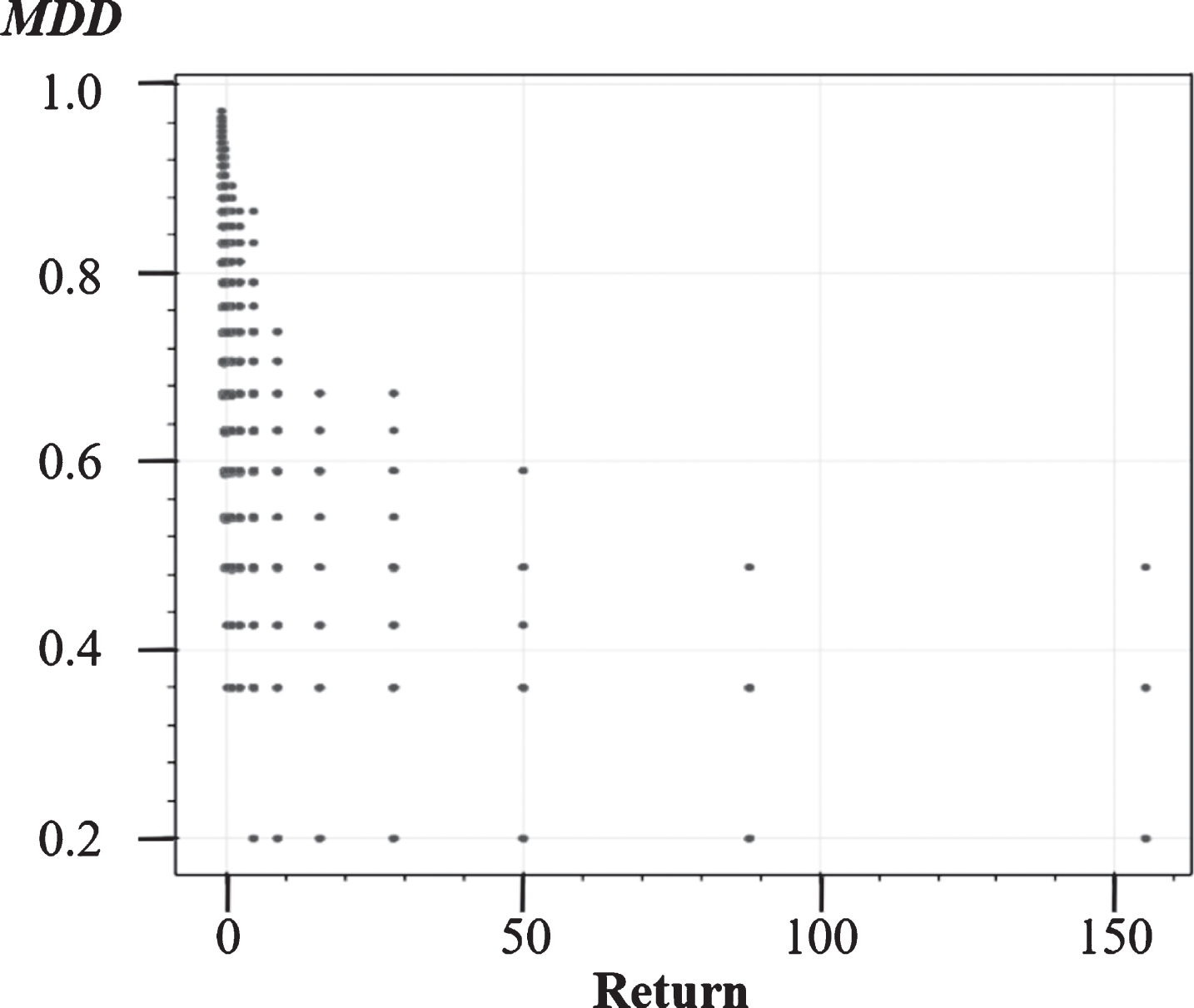
Simulation of single asset with f fixed at 25% and probability of winning fixed at 50% (i.e., odds of 2 and -1).
Here, we examined the influence of all the α combinations on returns when the fraction of assets to be invested is fixed at 25%. Each dot represents the result of one simulation. The overall simulation results revealed that the final MDD is inversely proportional to the final returns; i.e., a greater MDD means lower returns.
To summarize, within the confines of a coin toss, increasing the fraction of assets invested will lead to a concomitant increase in risk, which means that the maximum drawdown may also increase.
When dealing with a single asset, determining the relationship between the fraction of assets to invest and the probability of losing heavily is straightforward. By contrast, the complexity of portfolio optimization grows with an increase in the number of assets.
In the following simulation, we employed as our training dataset the FF48, which was developed by French and Fama in 1992. Note that these researchers gained widespread acclaim for their work in three-factor models and Fama went on to win the Nobel Prize in Economics jointly with Robert Shiller and Lars Peter Hansen in 2013. Thus, FF48 is considered the most credible and representative database in finance research, comprising stock data from 48 major industries listed on the NYSE, AMEX, and NASDAQ.
The parameters used in Algorithm 2 were aligned with the EGO portfolio, as follows: 50, 60, 60, and n0.5. Figures 4–6 present the results obtained using ensemble learning in which the subset method is used to improve the maximum drawdown. Figures 7–9 present the results obtained without subset sampling (i.e., using parameters 50, 60, 60, and n). The x-axis indicates the out-of-sample returns when applying the fraction of assets to be invested suggested by the proposed algorithm. The y-axis indicates the probability of MDD coming in at below a given risk target (α). As shown in Table 3, the results obtained using ensemble learning were superior to those obtained without. From this we can conclude that basing the configuration of Algorithm 2 on subset sampling (i.e., ensemble learning) increases the probability that MDD will fall below the loss limit stipulated by the investor.
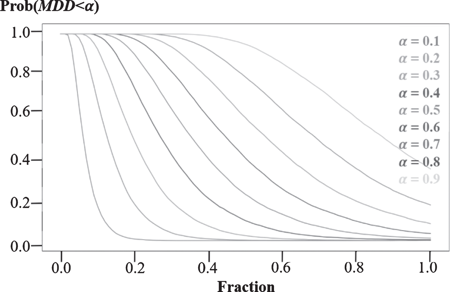
Simulation of single asset betting using odds sampling from a dataset with lognormal distribution, wherein mean and S.D. are 0 and 0.33, respectively.
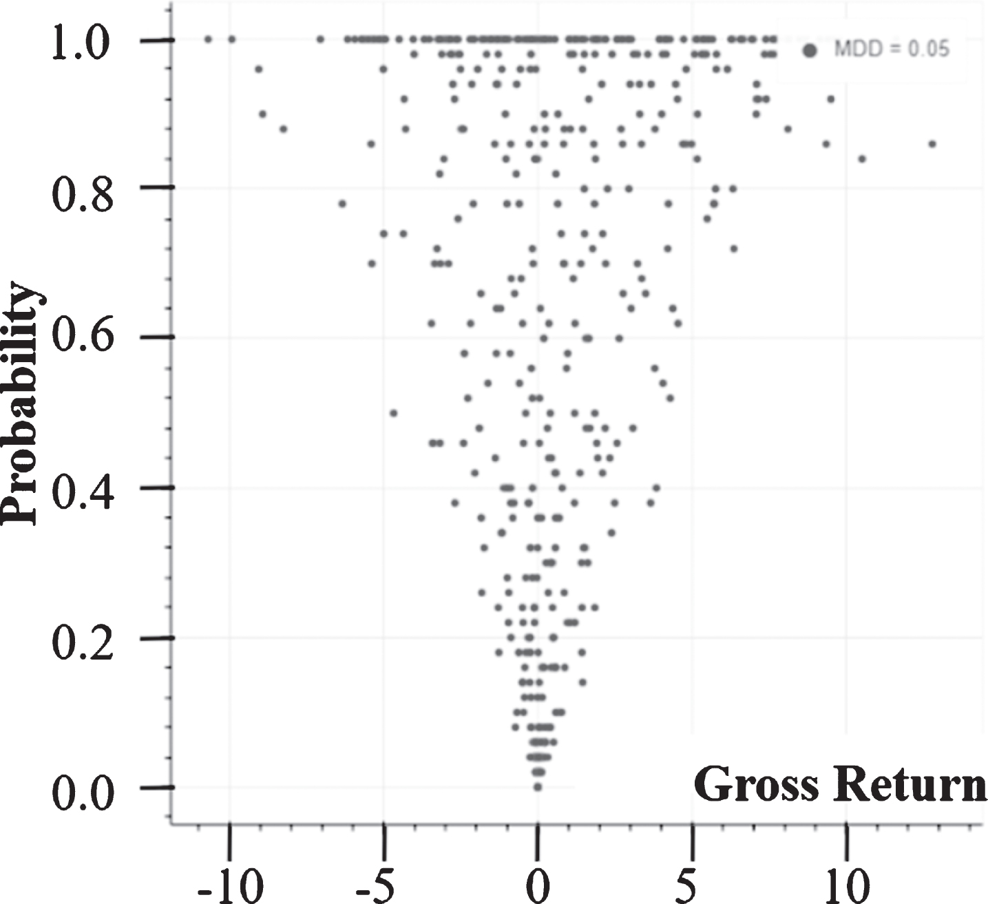
Simulation of multiple-asset optimization using ensemble learning and MDD of 5%.
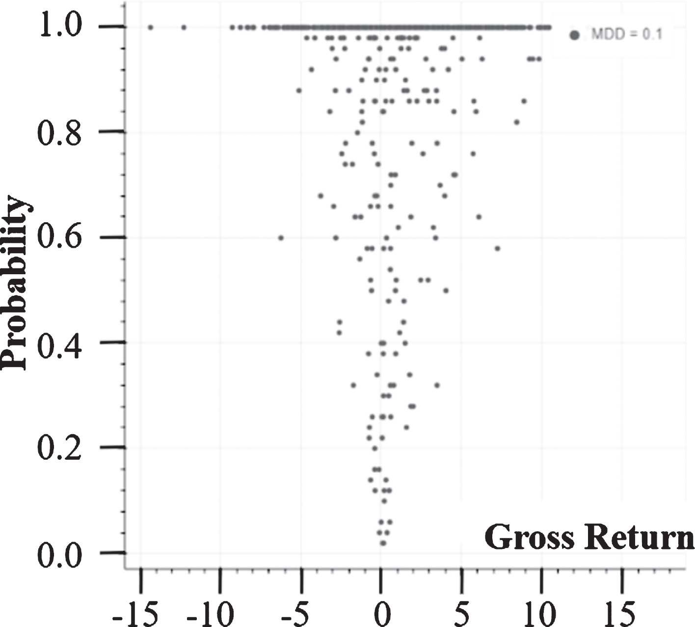
Simulation of multiple-asset optimization using ensemble learning and MDD of 10%.
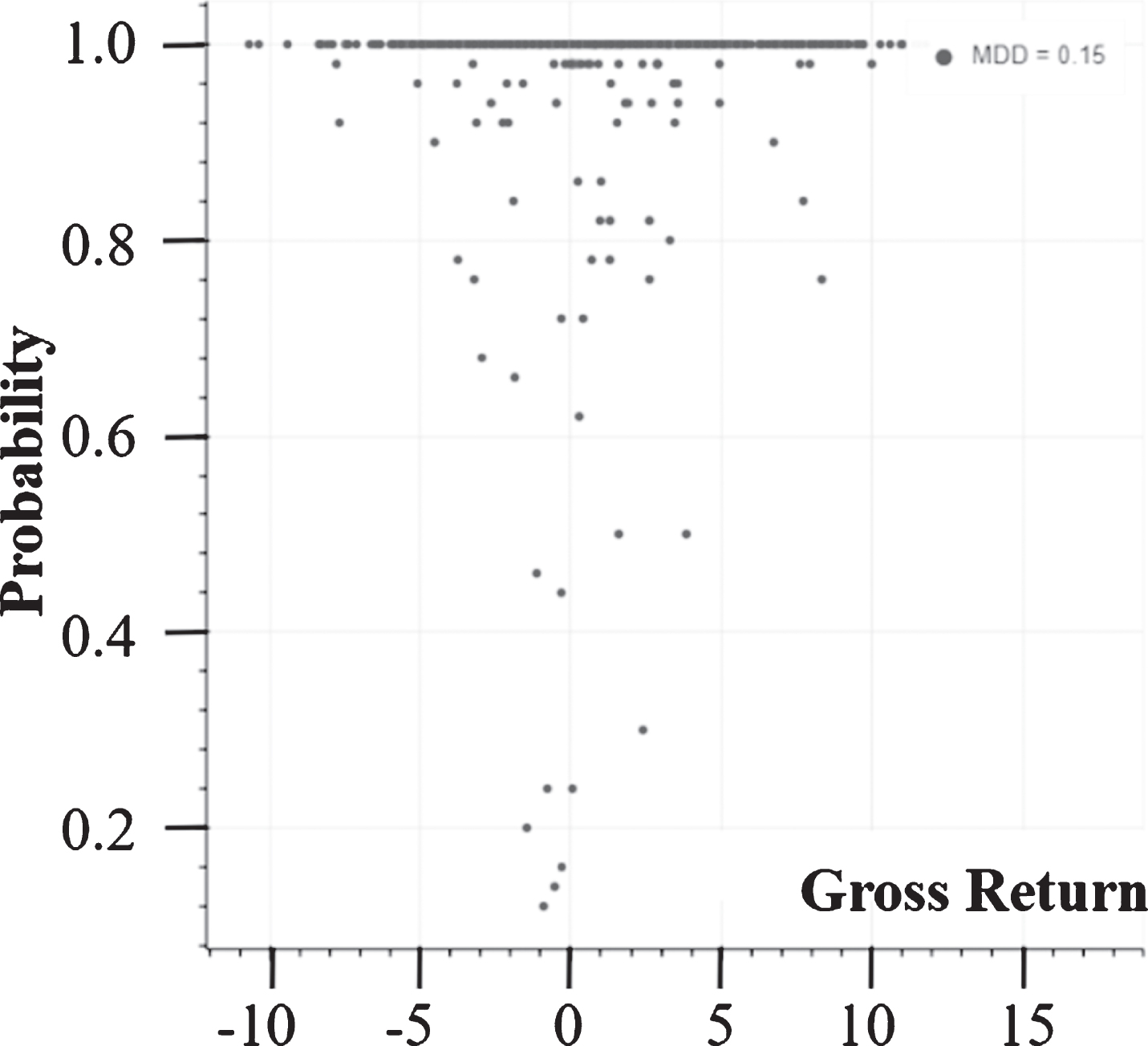
Simulation of multiple-asset optimization using ensemble learning and MDD of 15%.
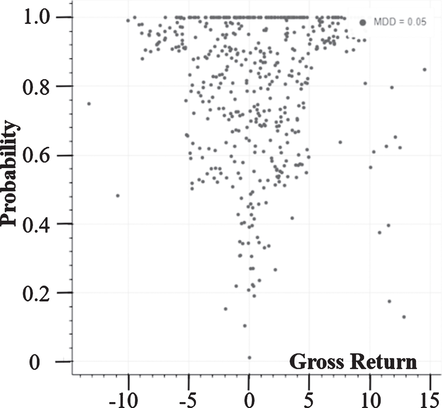
Simulation of multiple-asset optimization without ensemble learning and MDD of 5%.
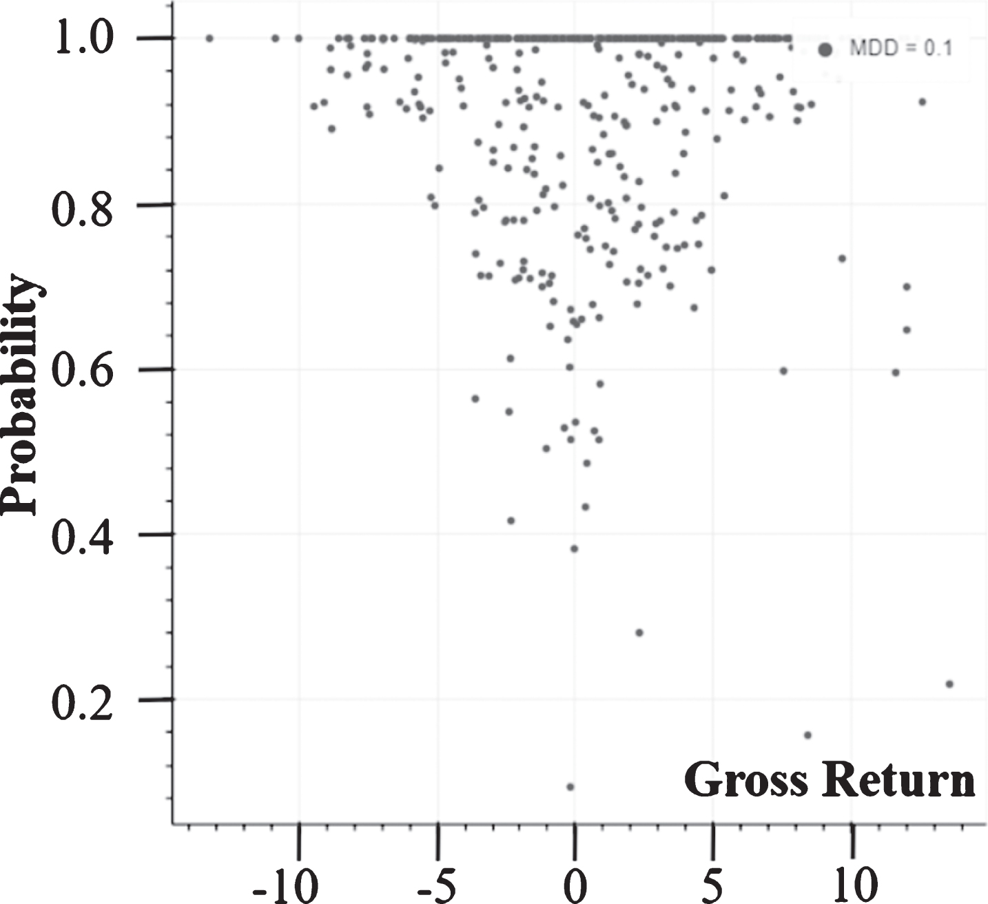
Simulation of multiple-asset optimization without ensemble learning and MDD of 10%.
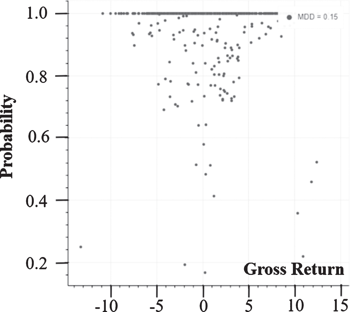
Simulation of multiple-asset optimization without ensemble learning and MDD of 15%.
Simulation with and without ensemble learning
Our objective in this study was to resolve the shortcomings of the conventional Kelly criterion by taking the maximum drawdown into account in order to prevent the probability of MDD falling below the level deemed acceptable by the investor. The first algorithm presented in this paper (based on Monte Carlo simulation) provides a systematic approach to determining the most suitable fraction of assets to invest in cases of a single asset. Our second algorithm (based on ensemble learning) is meant to optimize a portfolio within the constraints of a set gross return and set probability of experiencing losses beyond what the investor can bear. The current study was conducted using the FF48 dataset. In the future, we plan to present an online algorithm using the FF48 with moving windows to illustrate the performance of this algorithm in financial markets. It may also be possible to use neural networks to expand the scope of possibilities based on the fundamentals outlined in this paper.
Footnotes
Acknowledgment
This work was supported by the Ministry of Science and Technology, Taiwan, under Grant MOST 107-2221-E-027-104-MY2.