Many types of neutron spectrometer use a conventional primary spectrometer consisting of some collimator, a crystal monochromator and a second collimator. This article develops the description of the in-scattering plane component of the beam produced by such primary spectrometers using a graphical approach, 2D “Acceptance Diagrams”, for horizontally curved monochromators and a variety of collimator types (beamtubes, guides, conventional and radial Soller collimators). This visual approach clarifies the effect of primary spectrometer variables on the sample position beam. Conventional resolution descriptions use instrument parameter values to deduce the beam character produced at the sample and thence the full instrument transmission and resolution. This article solves the inverse problem of how to choose beam elements to deliver some desired beam character at the sample and shows that there are usually many equivalent choices. Dealing with this multiplicity seems to be a central issue in the search for optimal instrument designs, particularly if using numerical methods. The approach adopted here suggests a novel, mechanically simple primary spectrometer design offering great flexibility coupled with maximised transmission.
An accurate and complete description of the resolution of neutron scattering instruments is necessary both to analyse the data collected and to design better instruments. Extensive work has developed mathematical descriptions of the resolution of most significant types of neutron scattering instruments (e.g. Small Angle Neutron Scattering diffractometers (SANS), Constant Wavelength Powder Diffractometers (CW PD) and Three Axis Spectrometers (TAS) [1,2,13,16,17]). Usually, approximations are needed to make the description mathematically tractable so beams are often approximated as having infinite spatial extent and a Gaussian variation of transmission with angle to simplify the mathematics. This approach works because Gaussians are continuous smooth functions and both the product and the convolution of Gaussians are also Gaussian. Even so, the descriptions are so complex that it is now common to resort to Monte Carlo (MC) computer simulations [21,23,24] of instruments both for instrument design and the derivation of resolution functions. MC simulations are now also often used as the kernel of numerical optimization approaches to instrument design. A key issue in such studies is the choice of “quality factor” used to quantitatively compare results and the most advanced studies recognise the upper limit on performance imposed by Liouville’s theorem (e.g. [14]).
Many types of neutron scattering instrument (e.g. 4 Circle Single Crystal Diffractometers (SXD), CW PDs, TAS) use a conventional primary spectrometer (PS) consisting of a source, a collimator, a crystal monochromator and a second collimator. A full description of the sample beam requires a distribution of transmission, τ, from the source in a 5D space with the coordinates being horizontal (in-scattering-plane) and vertical spatial (x, y) and angular (γ, δ) deviations and wavelength or wave-vector (λ or κ). Such a complete specification makes any mathematical description or discussion complex and visualising or understanding effects in a 5D space is challenging. Conveniently, because there is effectively no γ–δ or λ–δ coupling in τ, horizontal and vertical effects are largely decoupled and can be treated separately. Vertical divergence effects have been described elsewhere [3–5] and are ignored in this work.
Conventional descriptions often remove any spatial variation from consideration by assuming a spatially infinite beam so the description becomes or . Some such approximation is needed to make the mathematics possible. Here, the infinite beam approximation is avoided by considering only the beam at the sample centre () and assuming that this represents the beam over the whole sample width accurately enough. MC computer simulations using McStas [23] show that this approach is usually quite accurate. The present work avoids relying upon the Gaussian approximation by using a graphical rather than a strictly mathematical approach. This use of DuMond Diagrams (DDs) [11] or Acceptance Diagrams (ADs), where beam transmission is plotted in an angle: wavelength () or angle: wave-vector () space, has been shown to be valid and to reproduce the known resolution results for CW PDs and TAS [7] but has remained on the fringe of neutron instrument design work. Presenting beam descriptions as 2D diagrams is well matched to the highly developed human capacity for processing visual images and so should be more immediately accessible and informative than a description expressed only by mathematical equations.
The use of vertical monochromator curvature to increase intensity is now widespread and it is becoming common to use horizontally curved or “focussed” monochromators (HFMs) as well. A large number of articles have discussed the resolution effects of HFMs on instruments and presented equations describing their effect (e.g. [18,19,22]). An earlier 3D (x, γ, κ) Acceptance Volume (AV) description of in-plane PS transmission [5] dealt with the restricted case of open beamtube collimation with HFMs but the 3D pictures are difficult to interpret and that work incorrectly interpreted guide transmission as acting like a virtual source (although the mathematical results and conclusions appear to be valid anyway).
This article develops a 2D description of PS transmission to the sample for a variety of collimator types (beamtubes, guides, Soller and Radial Soller) and for HFMs. This article identifies the primary spectrometer elements needed to produce a sample position beam with some desired character, a result needed for the analytic optimization of instruments. In some sense this is the inverse of the problem of describing instrument resolution for a given choice of beam elements. The presentation begins by defining conventions and symbols and describing 2D DDs and ADs for a PS using a variety of collimator and monochromator types. It is shown that the usual choice of components leads to over definition of the beam characteristics and mathematical relations are presented in Section 6 to describe and exploit this. A novel PS design is described which gives flexibility combined with maximised transmission, simple construction and simple control of beam parameters.
Problem outline, schematic, symbols and preliminary results
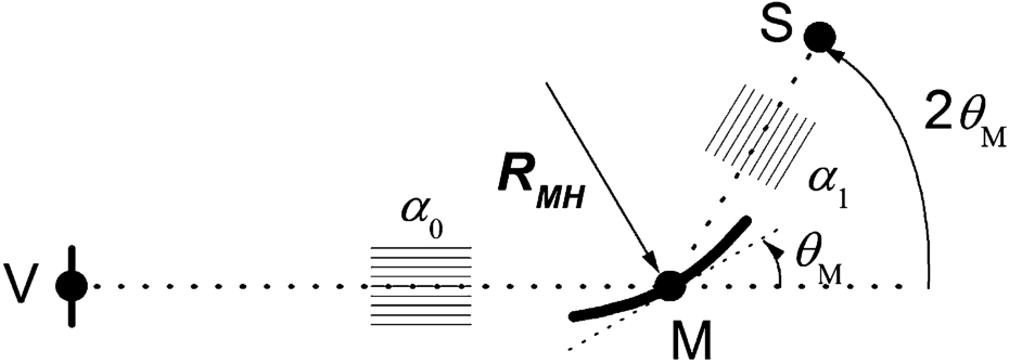
The conventional PS considered is illustrated schematically in Fig. 1.
Schematic diagram of the primary spectrometer discussed.
A (Virtual) source, at position “V” has width . This may represent the actual source or a slit placed somewhere between the actual source and the monochromator. A crystal monochromator, of width , is centred at position “M”, a distance from V, and is oriented at Bragg angle . The sample, at position “S”, is at a distance from M and the line from M to S makes an angle to the line joining V to M. is assumed to be much smaller than and so the monochromator’s projected width at source and sample is . Local right handed Cartesian coordinate sets with z along the beam propagation axis and y vertical are used at the significant points V, M and S in the PS. Individual rays have angular divergences from the beam axes of (between V and M) or (a variation in the scattering angle between M and S). The allowed divergences are restricted by beam collimators of half width (HW) or respectively. For collimators of Gaussian transmission profile , represents the full width at half maximum (FWHM). On neutron scattering instruments these angular divergences are invariably small enough that .
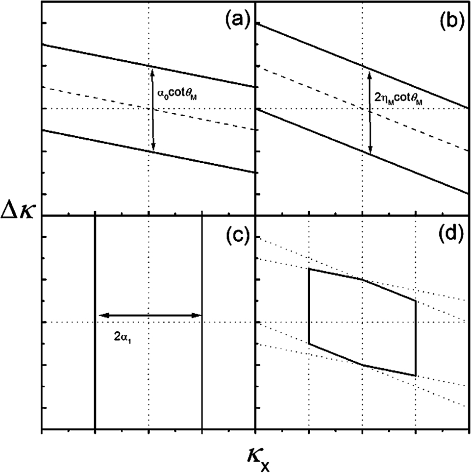
Visually, the AD description is clear and simple, as shown in Fig. 2. Describing the AD in words or mathematics is more complex and turgid. describes the distribution of transmission (usually equivalent to intensity) in the sample position beam in a 2D wave-vector space with coordinates and , . Equivalently, coordinates or (a DuMond diagram) can be used. is the product (superposition) of 3 separate AD’s associated with individual components – , & – and is bounded by an irregular hexagon as shown in Fig. 2(d).
This diagram illustrates the Acceptance Diagram view of the sample beam. The pictures describe the transmission in a 2D wave-vector space with x-coordinate the transverse wave-vector component and y-coordinate the variation from nominal longitudinal wave-vector component. The total transmission shown in Fig. 2(d) is the product of (Fig. 2(a)), (Fig. 2(b)) and (Fig. 2(c)) which describe respectively the transmission effects of the pre-monochromator collimator , the monochromator and the pre-sample collimation, .
For a mosaic monochromator, (for a Soller collimator or guide) is bounded by two parallel lines of slope which cross the axis at as shown in Fig. 2(a). For a radial Soller collimator or open beamtube the slope changes by a factor (). The transmission is modulated by the transmission profile.
(for a flat mosaic monochromator) is bounded by two parallel lines of slope which cross the axis at as shown in Fig. 2(b). Curving the monochromator in-plane changes the slope by a factor (). The transmission is modulated by the profile.
just limits the angular width () at the sample with no effect on the κ variation so it is bounded by two lines parallel to the axis which cross the axis at as shown in Fig. 2(c). Transmission is modulated by the profile.
The next sections of this article present equations which allow the pictures to be drawn accurately, show that the pictures truly represent the situation, and allow this graphical approach to be applied to instrument optimization.
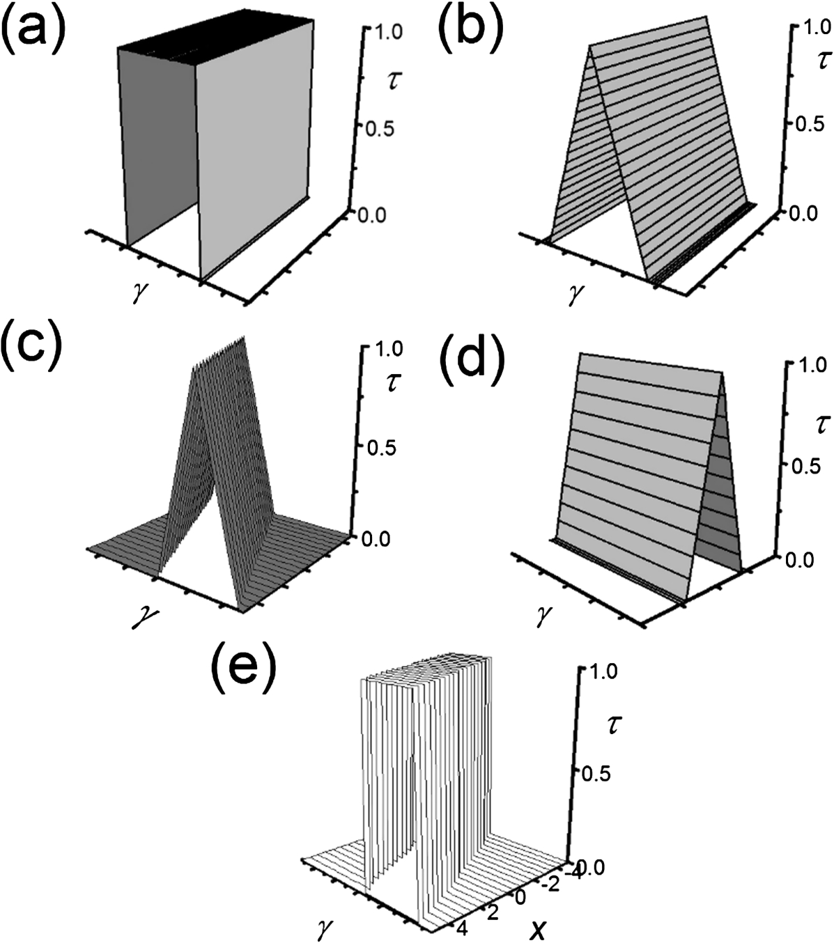
Phase space diagrams showing the transmission of various collimator types as a function of position and angle – the angle is proportional to the transverse wave-vector (or momentum) component. for (a) a guide, (b) a Soller collimator, (c) a diverging radial Soller collimator, (d) a converging radial Soller collimator and (e) an open beam tube or separated slit pair.
The transmission of individual PS beam elements
The transmission of different types of collimators (Soller collimators, idealised Straight Guides, Radial Soller Collimators and open beamtubes) is conveniently visualised using position–angle Phase Space Diagrams, , as shown in Fig. 3. All such collimators are insensitive to small variations in neutron wavelength. Strictly, a guide’s transmission angular width is proportional to wavelength but since the wavelength spreads considered here are typically less than 1%, this is a negligible effect. The transverse component of the wave-vector, , or neutron momentum is closely proportional to the angular divergence, γ, for small divergences.
Ideal long guides and Soller collimators produce beams where the angular divergence distribution is independent of position, x. Radial Soller collimators and open beamtubes produce beams with correlations between position and angular distribution.
An ideal long guide tube allows full transmission (%) up to some finite limit in space (guide width) and in angle ( where characterises the critical angle for the guide mirror coatings) as illustrated in Fig. 3(a). This effect can also be achieved in a short length using a reflecting Soller collimator. The mirror reflections may disrupt any existing angle-spatial correlations in the beam.
An ideal Soller collimator allows transmission which is spatially uniform with a triangular variation in angle, , as shown in Fig. 3(b). Note that this is an idealised representation as would be seen on averaging the beam over a spatial width much larger than a single collimator channel width.
The effect of radial Soller collimators depends on whether they are converging or diverging.
A diverging radial Soller collimator (as would be used between V and M) gives a triangular where the HW, α, is determined by the blade separation and length and the centre point of the distribution depends on transverse position x at distance as . This is illustrated in Fig. 3(c). Such a collimator effectively limits the source width visible.
A converging radial Soller collimator (as would be used between M and S) gives transmission independent of γ but with a triangular variation with position, , as illustrated in Fig. 3(d). Such a collimator effectively limits the beam spatial width at the sample.
For beamtubes, the local angular distribution is rectangular with constant width but the centre of the angular distribution varies systematically with transverse position.
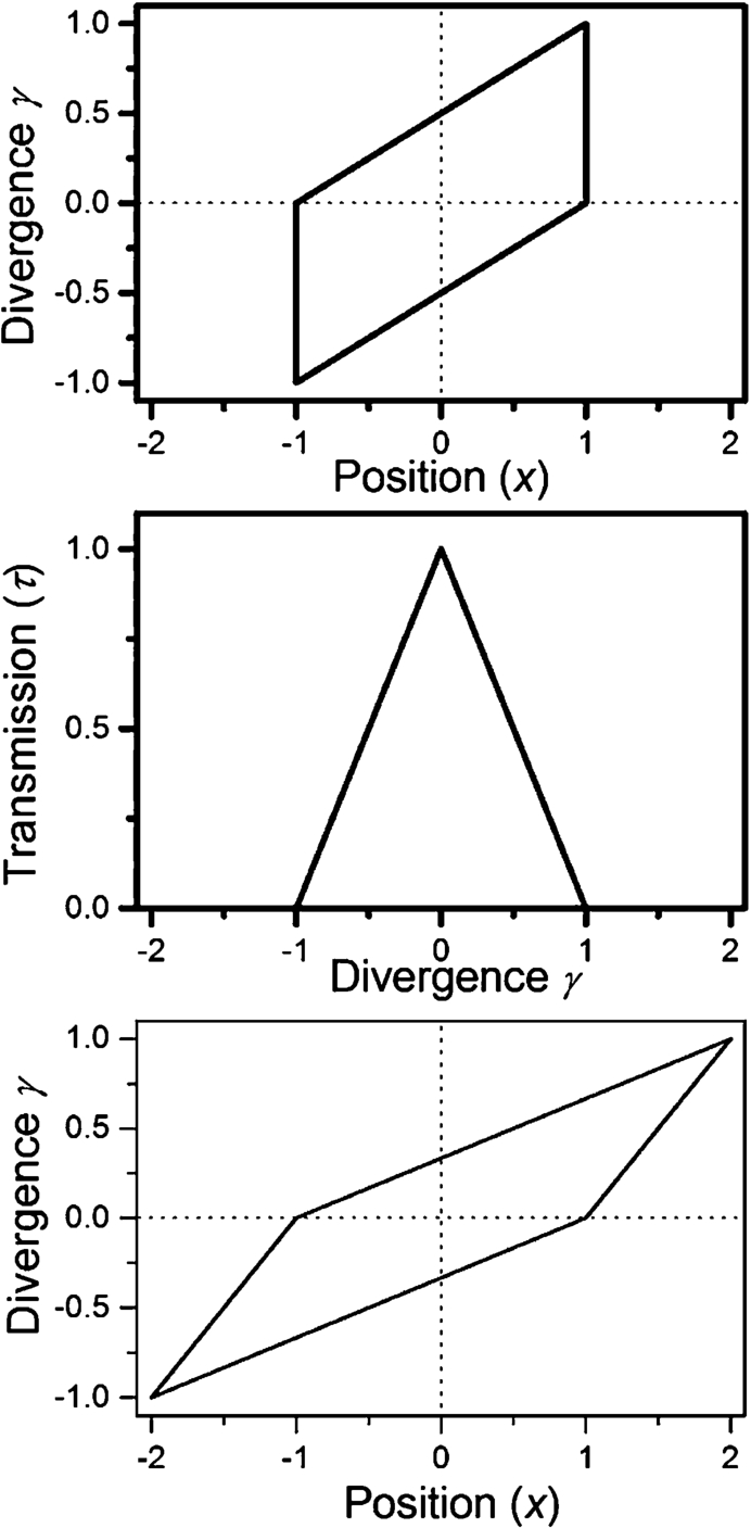
Transmission for an open beam tube (a separated pair of slits) here of equal width: (a) immediately after the second slit; (b) after the second slit; (c) some distance behind the second slit.
A diverging open beamtube (or a separated slit pair), as for between V and M, allows uniform full transmission at the monochromator for angles in the range as shown in Fig. 3(e) where is the x position along the monochromator surface. The illustration here is for a slit pair where the first slit is narrow and the second quite wide. For the case where the slits are of equal width, Fig. 4(a) shows the plot immediately after the second slit, Fig. 4(b) shows immediately after the 2nd slit and Fig. 4(c) shows Fig. 4(a) phase space diagram sheared as would be seen some distance behind the second slit.
A converging open beamtube, as for between M and S, gives % at the sample for angles where is the x position at the sample. This work only explicitly considers the beam at but it is simple enough to extend the results to finite .
Bragg scattering at the monochromator
A crystal monochromator scatters neutrons according to Bragg’s Law,
This gives the nominal scattered wavelength, λ, or wave-vector, κ, where is the monochromator lattice plane spacing and n is an integer (assumed to be 1). Combined with simple geometry, Bragg’s Law permits the calculation of the PS transmission as a function of angular and wave-vector divergence. Beams incident on a monochromator usually have some angular spread. Monochromator crystals are usually imperfect with a local “mosaic” or variation in crystallite orientation, η, often modelled by a Gaussian distribution of FWHM . Monochromator mosaic permits a variation in scattering angle and in wavelength or wave-vector. A d-spacing gradient, μ, a fractional variation in of up to , may also occur. A gradient allows scattering of different λ at a single Bragg angle.
The variation in Bragg angle is given by
where ξ is the local monochromator crystallite misorientation due to the combined effect of curvature and mosaic. Monochromator curvature can be regarded as “organised” mosaic (or mosaic as chaotic curvature) giving a systematic variation of ξ with position along the monochromator surface.
where is the monochromator radius of curvature. changes sign in passing the crystal due to the reflection and indicates that the x value before reflection is used. The scattering crystal element must have whence . To solve the ray tracing equations and proceed with the analysis some restriction must be applied and usually this is to assume a uniform beam of infinite width. Since this assumption cannot be justified for HFMs or converging or diverging collimators or beamtubes, it is replaced here by considering only rays reaching the sample centre, , when
Often, the beam at is representative of the beam over the whole sample width but, if this is likely to be important to the measurement considered, this can be checked either by an MC simulation or by calculating the beam character for .
DuMond diagrams for conventional primary spectrometers
This section presents 2D diagrams in a space (DuMond) illustrating the effect on the sample position beam of the elements of conventional primary spectrometers using flat monochromators (Fig. 5). The reciprocal space formalism of Von Laue is more powerful and general but it is usual to first learn diffraction theory in the Bragg formalism expressed in angles and wavelengths and many experienced users of diffraction instruments continue to think naturally in this way. In this section, it is assumed that all elements have rectangular transmission profiles – so transmission is 100% up to some limit where it falls to 0%. The scattered beam is considered at the point which is assumed to be representative of the beam over the sample width of interest. Thus, the beam within the PS is assumed to be sufficiently wide that spatial effects can be ignored. The monochromator is assumed to be flat and oriented at an angle to the nominal incident beam direction. Local variations in crystal mosaic element orientation (η) or incident ray direction () alter the effective Bragg angle to and the angle between the incident and scattered rays to .
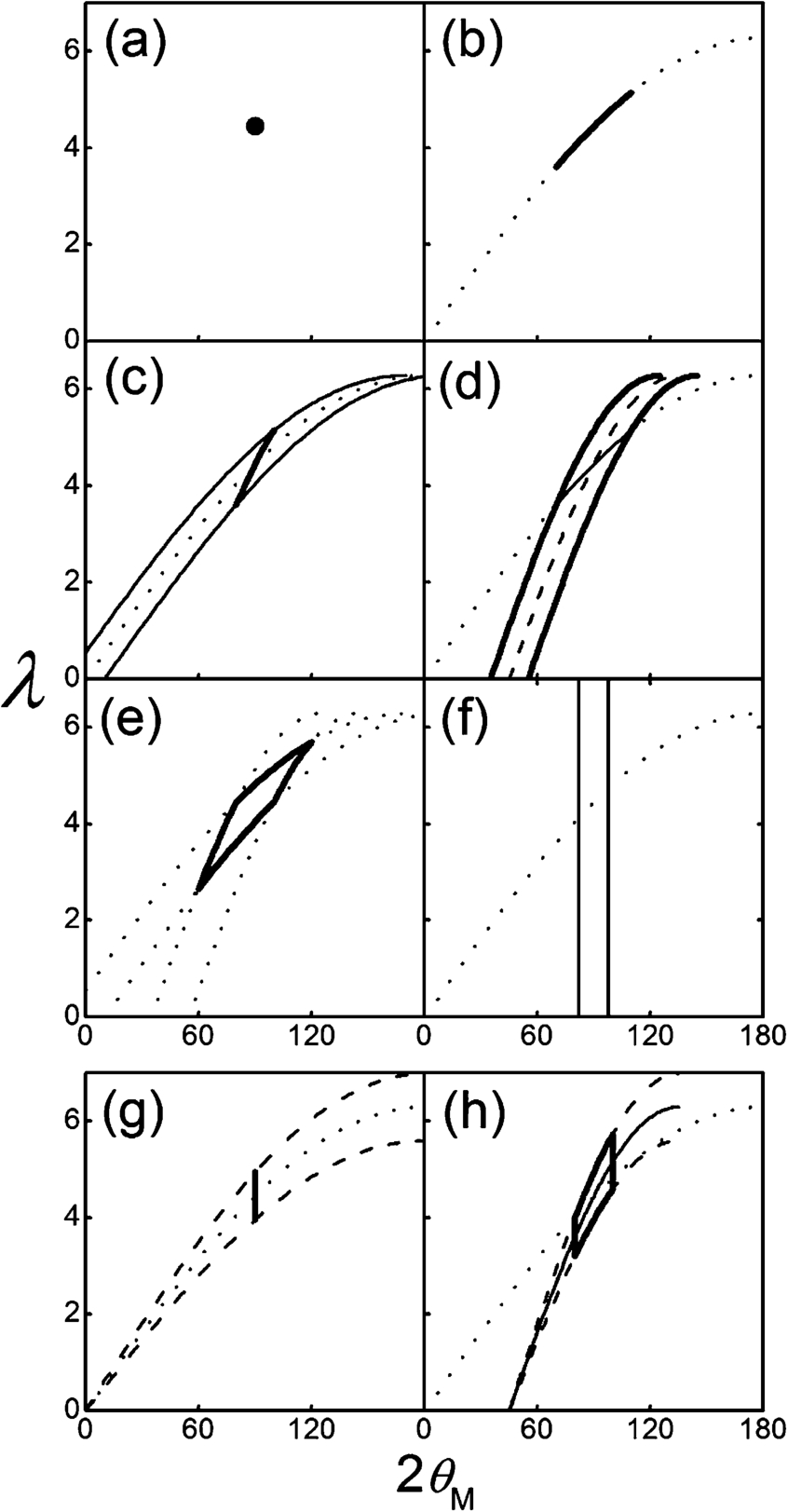
For a perfectly collimated “white” incident beam containing all wavelengths, a flat monochromator crystal of zero mosaic oriented at Bragg angle produces a monochromatic beam at scattering angle . The DuMond diagram for this situation shows a single point of intensity (Fig. 5(a)). A scan of that monochromator (or alternatively, using a monochromator where the mosaic is , i.e. a powder) produces the familiar curve of wavelength variation with scattering angle shown by the dotted line in Fig. 5(b). For an un-scanned monochromator with finite mosaic, intensity appears along a segment of that curve as shown by the solid line segment in Fig. 5(b).
If a “monochromator” with mosaic is now illuminated by a perfectly collimated white beam displaced by some small angle, , from the incident beam axis, the curve is also displaced by parallel to the axis. It follows that if the incident beam has some finite angular width, , the curve is broadened by parallel to the axis as in Fig. 5(c). The effect of such a beam angular width on a monochromator with zero mosaic is illustrated by the short solid line segment.
Now consider a flat crystal monochromator of zero mosaic at orientation illuminated by a “white” beam with all divergences between glancing and normal reflection from the monochromator. Rays will be diffracted with incident Bragg angles varying from 0° (scattered angle ) to back scattering (scattered angle °) with corresponding variation in wavelength as shown by the dashed line in Fig. 5(d). The effect of finite monochromator mosaic is shown by the short solid line segment and this results in broadening the dashed curve as shown by the solid lines in Fig. 5(d).
Combining the effects of finite mosaic and incident beam divergence gives an acceptance area on the DuMond Diagram as shown in Fig. 5(e). This defines the range available in the beam following the monochromator. The effect of collimation between the monochromator and the sample, , is to limit the angular range of rays visible at the sample as shown in Fig. 5(f).
Figures 5(c), (d) & (f) illustrate the transmission allowed by each element. The total transmission is all rays which can pass all three PS elements i.e. the product or superposition of these three DuMond Diagrams corresponding to the individual PS elements.
Now, consider a gradient crystal monochromator with zero mosaic but a range of d-spacings, described by a fractional variation , such that . A perfectly collimated incident white beam is scattered at a single angle but with a range of wavelengths as shown by the short vertical solid line in Fig. 5(g). The dashed lines show how this wavelength range depends on Bragg angle, as would be seen in a rocking scan. Notice that for a gradient monochromator the wavelength spread is larger at large , i.e. large wavelengths () in contrast to the reduced wavelength spread at large scattering angles and wavelengths seen with mosaic monochromators (). This suggests that in some applications gradient monochromators would have an advantage for short wavelength neutrons where is usually small leading to a large and poor λ resolution. Attempts have been made to construct gradient monochromator crystals for many years with limited success (e.g. [15]). It may be possible to manufacture composite gradient crystals from a stack of thin crystal plates each with slightly different concentration and hence d-spacing (made, for example, using a “micro pull down” furnace [20]). Elastically bending crystals induces a lattice spacing gradient so if necessary the stack of crystal plates could be bent slightly to make the d-spacing gradient continuous rather than discrete. The clever use of slabs of the comparatively cheap and readily available large crystals of near perfect silicon or germanium manufactured for the semiconductor industry as bent neutron monochromators is now relatively common. The AD formalism should apply to such monochromators, at least approximately. For such monochromators the degree of gradient induced is coupled to the monochromator curvature which is often adjusted when is changed.
Figure 5(h) shows the effect of a white beam with angular width incident on a gradient monochromator. The solid lines outline the DuMond diagram for finite while the dashed lines show the effect if . Because in scattering from a flat gradient monochromator, has the same effect as .
The spreads in angle and wavelength for neutron primary spectrometers are typically quite small (of order 0.5° or 0.5%). Under these circumstances, the curvature of the lines bounding the DDs becomes insignificant and they can be represented accurately enough as straight lines. In this limit, starting with a perfectly collimated incident beam, , and a monochromator for which :
A spread in broadens the 2D DuMond diagram point by
Monochromator mosaic broadens the DuMond diagram point by
Monochromator d-spacing gradient broadens the DuMond diagram point by
Angular collimation in the scattered beam limits the DuMond diagram by lines at
Acceptance Diagrams for individual PS elements
The conventional primary spectrometer considered here is itself a diffraction instrument and the viewpoint most likely to be informative is a wave-vector space. The DuMond diagrams in Section 3 can be equivalently presented as , the sample beam Acceptance Diagram drawn in an angle: wave-vector space. The AD plotted in a space is just the reflection in the γ axis of the DuMond diagram plotted in a space.
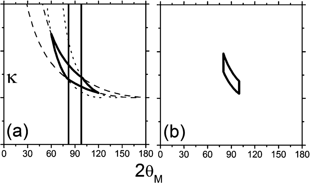
This section develops expressions describing the AD limits in wave-vector space for different types of collimating elements and for curved as well as flat monochromator crystals. It is assumed that the monochromator is thin and that any curvature is continuous although in practice the curvature is usually achieved approximately using small oriented crystal segments. Figure 6(a) shows and its component parts for individual PS elements corresponding to Figs 5(c), (d) & (f). Figure 6(b) shows for the gradient monochromator case corresponding to Fig. 5(h).
Acceptance Diagrams – plots of : (a) for finite ; mosaic monochromator with finite ; (b) for finite ; gradient monochromator with finite .
A small angular variation from the nominal beam direction at the sample, , equates to a small fractional variation in , the x-component of the wave-vector (). If is small, then and thus . Formally, represents in spherical polar coordinates or in Cartesian coordinates. For mathematical convenience, the representation used here is which displays equivalent information. The beam is assumed to be sufficiently spatially uniform over the sample for any non-uniformity to have negligible effect on measurements (usually a necessary condition for sensible measurements) so spatial variations are largely ignored. Achieving this in practice usually simply requires “sufficiently large” PS dimensions.
Assuming that all divergences are relatively small, for the case of rectangular profile collimators with a flat mosaic monochromator considered in Section 3, is bounded by three pairs of straight lines:
For a gradient monochromator is bounded by two pairs of lines:
Just as the sample position DD is the product of three component DD’s, so is the superposition or product of three AD’s corresponding to the effects of the collimation, the monochromator and the collimation denoted , and .
It is simpler and clearer to consider as this product than as a single whole.
and depend on scattering at the monochromator which allows a range in wave-vector given by equation (2). The derivations are conducted here only for beamtubes delivering rectangular angular profiles but non rectangular angular profiles can be superimposed later as a modulation of τ along well defined directions. Setting describes the guide and Soller collimator cases.
for a mosaic monochromator
includes all neutron rays which can reach regardless of the values of , and . is derived by assuming that is large enough that all incident rays allowed by can be scattered at the monochromator. Consider an open beamtube between V and M with a fully illuminated (virtual) source so that rays reach all parts of the monochromator. Then the “global” incident divergence is at least but at each point on the monochromator, the “local” angular spread is which may be much smaller. The centreline of is calculated by setting ; for a beamtube this is achieved by setting the source width to zero. Then, and applying equations (3c) and (5) yields
This describes a line of intensity in . Introducing a finite broadens this line in along a direction calculated by now setting . Applying equations (2), (3a) and (4) yields
Equations (3a), (3b), (4) and (5) show that and so that the limits of this broadening line are set by the value of as . Calculating at the end of this broadening line and subtracting the value of at the centreline there gives a broadening of regardless of the values of or . Thus, is the region bounded by the lines
The extent of may be restricted by the values of and .
for a gradient monochromator
For a gradient monochromator, , so a ray can only scatter if where . lies in the range with . The effect of is simply to restrict the range of with limits as before. Note that this also affects the sample beam spatial size which is limited to if the monochromator is fully focussed from source to sample. For a flat monochromator the sample beam width is limited by the source and monochromator widths and the allowed beam divergence.
includes all neutron rays which can reach regardless of the values of , or . Assuming that is unrestricted and conducting the derivation as before for a curved monochromator on a beamtube, the centreline is calculated by setting when . Applying equations (3a) and (5) yields
A finite broadens this line along calculated by setting so that at , . The limits to this broadening line are set by (or if not, by or ). The equality shows that lies in the range . Calculating at the end of this broadening line and subtracting the centreline there gives a broadening of regardless of or . A curved monochromator can be regarded as having small mosaic segments selected in some organised way from the of some larger mosaic flat monochromator.
A monochromator d-spacing gradient broadens the line by with the limits given above.
The broadening effects of: (a) on . centreline is found by setting and . For flat monochromators (illustrated here) broadening has extent ( axis) along . (b) on . centreline is found by setting and . For flat monochromators as here broadening is ( axis) along .
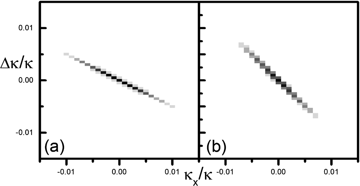
Figure 7(a) illustrates the broadening effect on of with the centreline of indicated by the dashed line (here °). Figure 7(b) shows the broadening effect on of with the centreline shown by the dashed line (again, °). Figure 8(a) shows a McStas simulation of the sample position beam from a PS using a flat monochromator with and a very small (). This gives an which follows the broadening line. Figure 8(b) shows a simulation of beam with and a very small () showing the broadening line. These simulations confirm the mathematics.
McStas simulations showing illustrating the broadening effect of (a) on where with ; (b) on where with .
– collimator between the monochromator and sample
Beam collimation between the monochromator and sample plainly has no effect on wave-vector and simply restricts the sample beam’s angular divergence distribution. consists of equi-transmission contours parallel to the axis with the profile, , dependent on the type of collimation. At the angular distribution is triangular for a Soller collimator and rectangular for an ideal guide with . For a beamtube or converging Radial Soller collimator, the angular distribution at is rectangular with where . The illuminated monochromator width sets an upper limit of on angular width for all collimators.
In this discussion of AD shapes, no consideration has been taken yet of the absolute value of the “transmission”. The transmission at each point in should be 100%, multiplied by any losses due to collimator transmission, monochromator reflectivity, air scattering or absorption by any windows in the beam. The transmission must be modulated along the individual AD axes by consideration of any transmission profile due to or collimation or to monochromator mosaic. The total beam flux at (clearly ignoring vertical divergence effects) is the source flux multiplied by the integral of τ over . Thus, the intensity depends on the Acceptance Diagram area so that a larger AD, corresponding to a beam with large angular and wave-vector spreads, represents a higher intensity with correspondingly reduced resolution. The instrument count rate will be proportional to this intensity multiplied by the sample area.
Sample position Acceptance Diagram in the Gaussian approximation
This section discusses the product for “Gaussian” elements, an approximation often applied to triangular transmission functions. Considerable work and many publications have been devoted to deriving the full resolution function for many types of neutron scattering instruments including those using HFMs. This section is not intended as any replacement for any existing formalism (e.g. [2,17,18,22]) but simply as a bridge from the pictorial view described in Sections 2, 3 and 4 to the significant results sought in Section 6.
To generate (approximately) Gaussian profiles in each PS component, consider a PS using a Radial Soller collimator for , a Gaussian mosaic HFM and a conventional Soller collimator for . The individual transmission functions are then
with the factors in each Gaussian allowing , and to be written as FWHM. , the total AD at the sample centre, , is the product of Eqs (10a), (10b) and (10c) and is
where
Equation (11a) should include transmission terms to account for any beam losses in the PS but these are all assumed to be 100% here. Fixing τ in Eq. (11a) to some value gives an elliptic contour of constant transmission probability. The significant contour at ,
intersects the axis at
intersects the axis at
has maximum extent in the direction of
has maximum extent in the direction of
has angle between the -axis and the ellipse axis of
The known and well tested expressions for CW PDs and TAS resolution using Soller collimators and flat monochromators can be recovered from Eq. (11a)–(11b) by setting when
This should give confidence in this extension of the AD description to non Gaussian collimators and HFMs. Equation (11a)–(11c) for the PS AD should be directly transferrable to the known expressions describing the resolution of CW PDs and TAS permitting the inclusion of HFMs in existing resolution formulae.
Note that altering by varying either or for a radial Soller collimator shears parallel to the axis. Altering shears parallel to the axis but does not affect the area of . Adjusting either or affects the overlap between and showing that increased intensity at the sample from horizontal monochromator curvature results from better matching to giving access to a larger range. That effect is maximised when the slopes of and are exactly matched which corresponds to the well known source to sample “focussing condition” for a HFM when
If is a guide (), then and if (the “monochromatic” focussing condition), then . If the monochromator curvature takes the Eq. (12) value,
and
The equations suggest that if the monochromator curvature is convex rather than concave, then the slope of increases and, presumably, matching this would require a convergent rather than divergent beam before the monochromator.
Relationship between instrument parameters and
This section discusses the range of PS parameters which can be used to deliver some chosen beam characteristics.
Within a Gaussian approximation, the values of (Eq. (11b)) can be used to draw elliptical contours of constant transmission probability in as described in a or space. As far as scattering by the sample is concerned, any beam of a given κ with identical values for the variables (A, B, C) has an identical effect. The description would be more useful in discussing instrument resolution if it used parameters simply related to the observed scattering. It is useful to consider a “delta function scatterer” sample which transforms incident neutrons by some fixed . Such a sample represents a Bragg peak in the elastic scattering case (where ). For Bragg peak sample scattering, equation (2) can be adjusted to become showing that scattering shears parallel to the γ axis. A useful parameter set to describe , at least for CW PDs, proves to be as illustrated in Fig. 9.
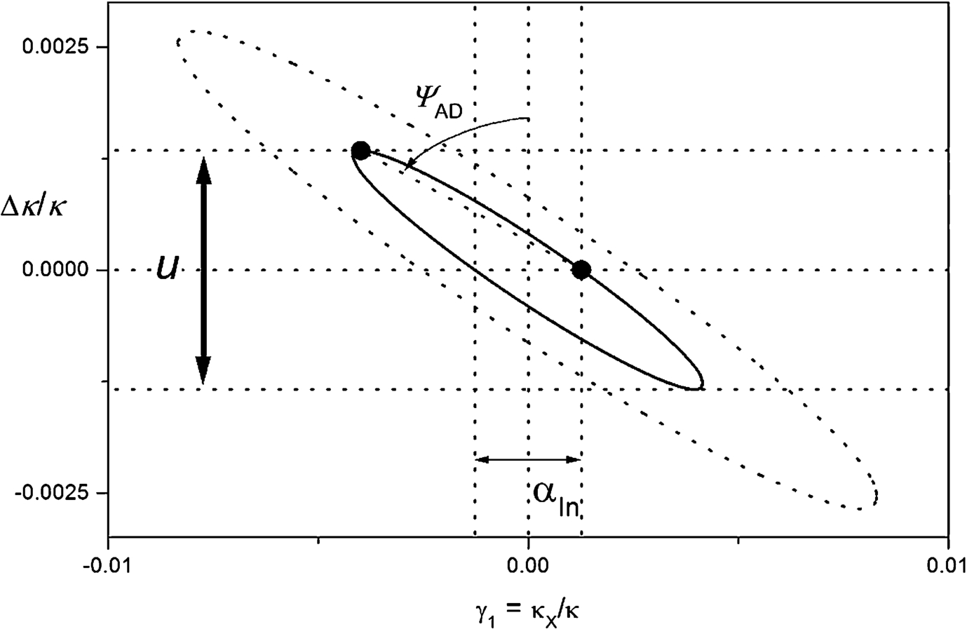
Illustration of a primary spectrometer arising from Gaussian profile collimators and mosaic showing u, ψ & with their extent indicated by dotted lines. The two ellipse contours represent the 50% and 6.25% transmission contours.
Here is the beam angular width (FWHM) at the nominal wave-vector measured at the axis. u is the maximum extent (FWHM) of the elliptical contour in the direction. is the angle between the axis and the line joining the origin to this point of maximum extent. Note that is negative for positive . The parameter u is equal to where U is the first of the parameter set (U, V, W) commonly used in Rietveld analysis of powder diffraction patterns. u describes the degree of peak broadening arising from wavelength spread in the beam. In the Gaussian model, determines the scattering angle on a PD at which the peak width is smallest. These parameters can be seen to be related to the notion that on a PD the in-plane contribution to peak broadening arises from a combination of wavelength spread and angular spread in the incident beam. It is straightforward to show that
It has been shown [8] that many values of (, , , ) can deliver identical resolution on CW PDs within the Gaussian approximation for a PS using Soller collimators and a flat mosaic monochromator. Such parameter sets all have the same detector collimation so this parameter multiplicity is plainly associated only with the PS. If the desired beam character is known, then, starting from equation (11b) and the known values for (A, B, C) or (u, , ), parameter values can be deduced which deliver that beam in the more general case discussed here which allows for HFMs and open beamtubes. The mathematics defines 3 functions of 7 parameters and deducing the relations requires fixing 4 of the parameters. There are many combinations of parameters which could be fixed but only three cases are treated here. The first case considers conventional Soller and collimators with a flat mosaic monochromator (fixing , , ). The second case considers conventional Soller or guide and collimators with a mosaic monochromator curved to focus from source to sample (with and fixed). The third case uses a radial Soller for , a curved mosaic monochromator and a conventional Soller collimator for with the axes of and aligned (fixing , coupling and and coupling and ). In the first and third cases, is used as a variable to display the range of values possible.
Soller collimator and with flat mosaic crystal monochromator
The case of a conventional primary spectrometer using Soller collimators for and and a flat mosaic monochromator crystal corresponds to setting . Then it is straightforward starting from Eq. (11b) and fixing to show that
Applying equation (14) shows that
Instrument parameters can be found to deliver the sample position beam described by or for a range of values. That allowed range can be found using the requirement that , and all be positive; so
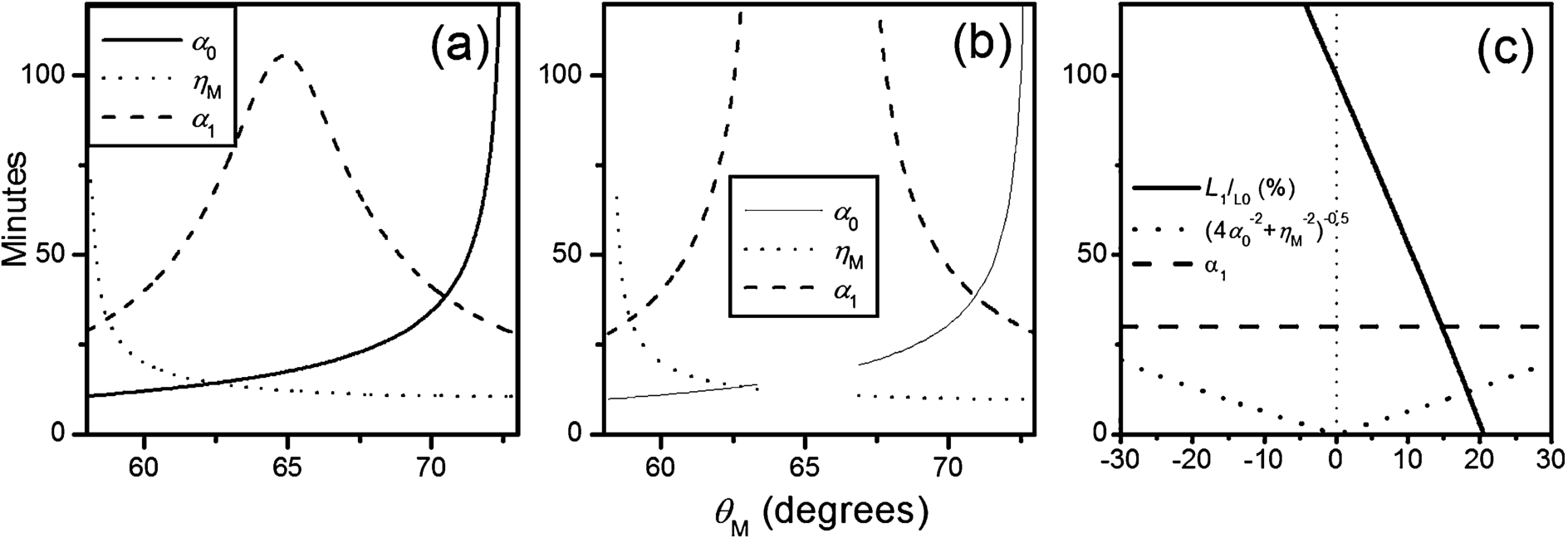
The allowed range is often continuous but sometimes has a disallowed mid-region where would be negative. One approach to choosing suitable values for instrument variables is to calculate and plot values for , and over the allowed range of and then choose a value for which the set of variables is technically convenient. Figures 10(a) and 10(b) show examples of the allowed values.
(a) Values of vs for given (A, B, C) in a Soller-flat mosaic-Soller PS. The values shown here deliver a beam identical to that for . (b) Values of vs for given (A, B, C) in a Soller-flat mosaic-Soller PS. The values shown here deliver a beam identical to that for . Note the split in the allowed range of . (c) Values of , and vs for given (A, B, C) in a Radial Soller-curved mosaic-Soller PS. Here the beam delivered matches that for Fig. 9(a).
Soller collimators or guides using a focussed monochromator to align and
It is possible to curve the monochromator in the scattering plane and thus increase the alignment of and which should improve the PS transmission. The case of a conventional primary spectrometer using Soller or guide collimators for and and a curved mosaic monochromator focussing to the sample corresponds to setting and . Then it is straightforward starting from Eq. (11b) and fixing to show that
It follows that
Here there is only one allowed value for but multiple values of and so can be chosen to match some preferred value.
If using Soller collimators, the distributions and are triangular. If using an ideal guide before the monochromator, becomes rectangular. It is possible to use a slit defining the beam width either just before or just after the monochromator to set the value for and give a rectangular distribution. Choosing rectangular distributions should increase transmission for a given resolution. In this case, the centre of varies with position at the sample; which may or may not have a significant effect on scans.
Focussed monochromator with and aligned
For a PS using a radial Soller , curved mosaic monochromator and conventional Soller , matching the and slopes and fixing yields
It follows then that
In this case, always takes the same value for given (A, B, C) regardless of the value of . The sum () is the significant variable so the individual values of and can be varied freely as long as this sum remains constant. Figure 10(c) shows an example of the allowed values for a single choice of (A, B, C). The limits to are set by the requirement that be positive, so . Note that solutions exist for a reversed sign of when .
It is desirable to choose beam elements to deliver rectangular transmission profiles in to increase transmission for given instrument resolution. This can be done using open beamtubes between virtual source and monochromator where the virtual source width sets and between monochromator and sample where the effective monochromator width, which could be controlled by a slit just before or just after the monochromator, sets . To achieve the same resolution variance for a PS using rectangular elements the HW values for , and should be approximately times smaller than the Gaussian FWHMs. The relations presented above can be regarded as indicative of appropriate values for rectangular profile elements but should be used with some care. For example, for an with rectangular transmission profiles, the proper value for for a CW PD is probably the angle from the origin to the upper left vertex of , i.e. where β is the smaller of and .
Some examples of equivalent primary spectrometers
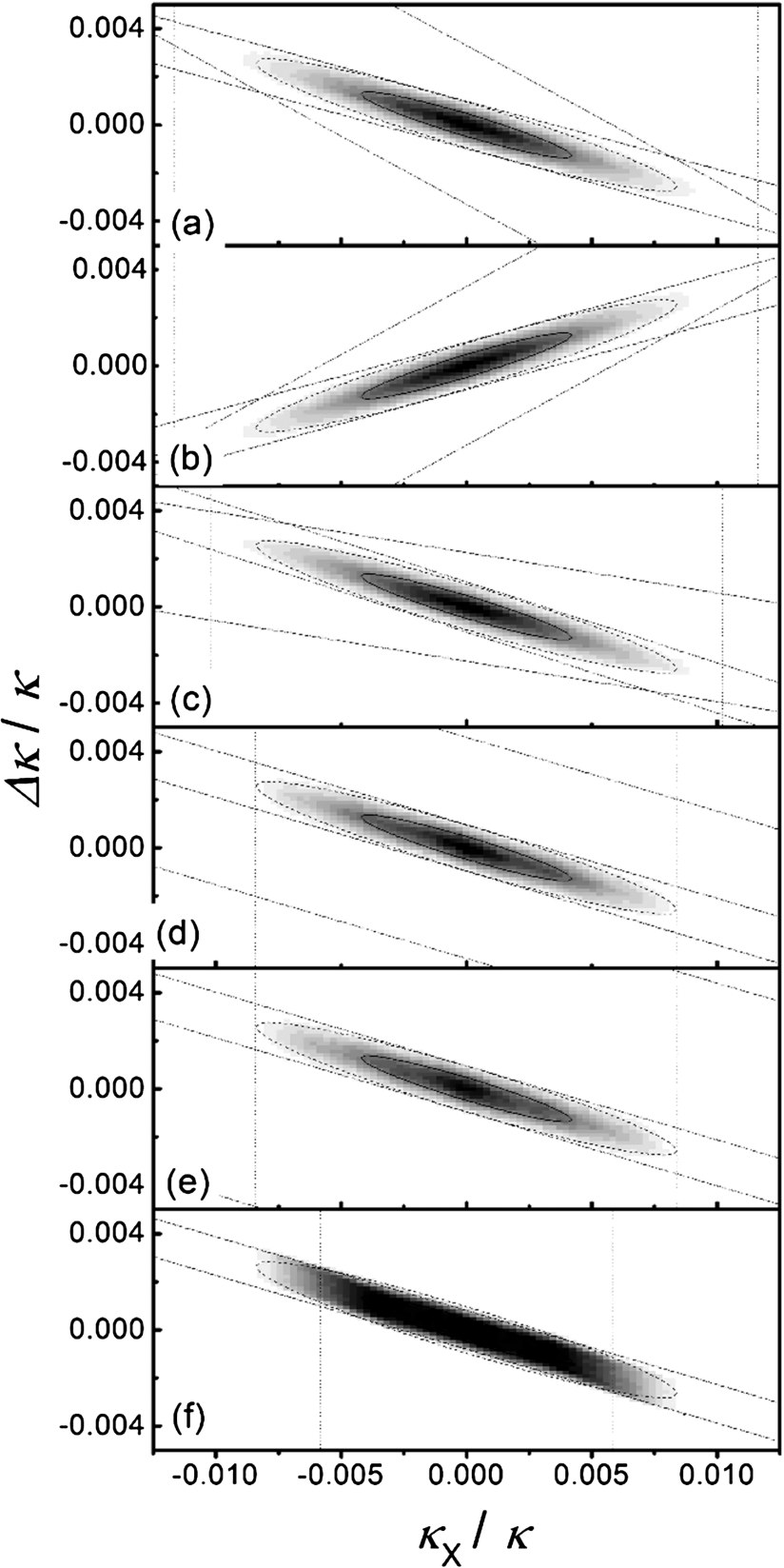
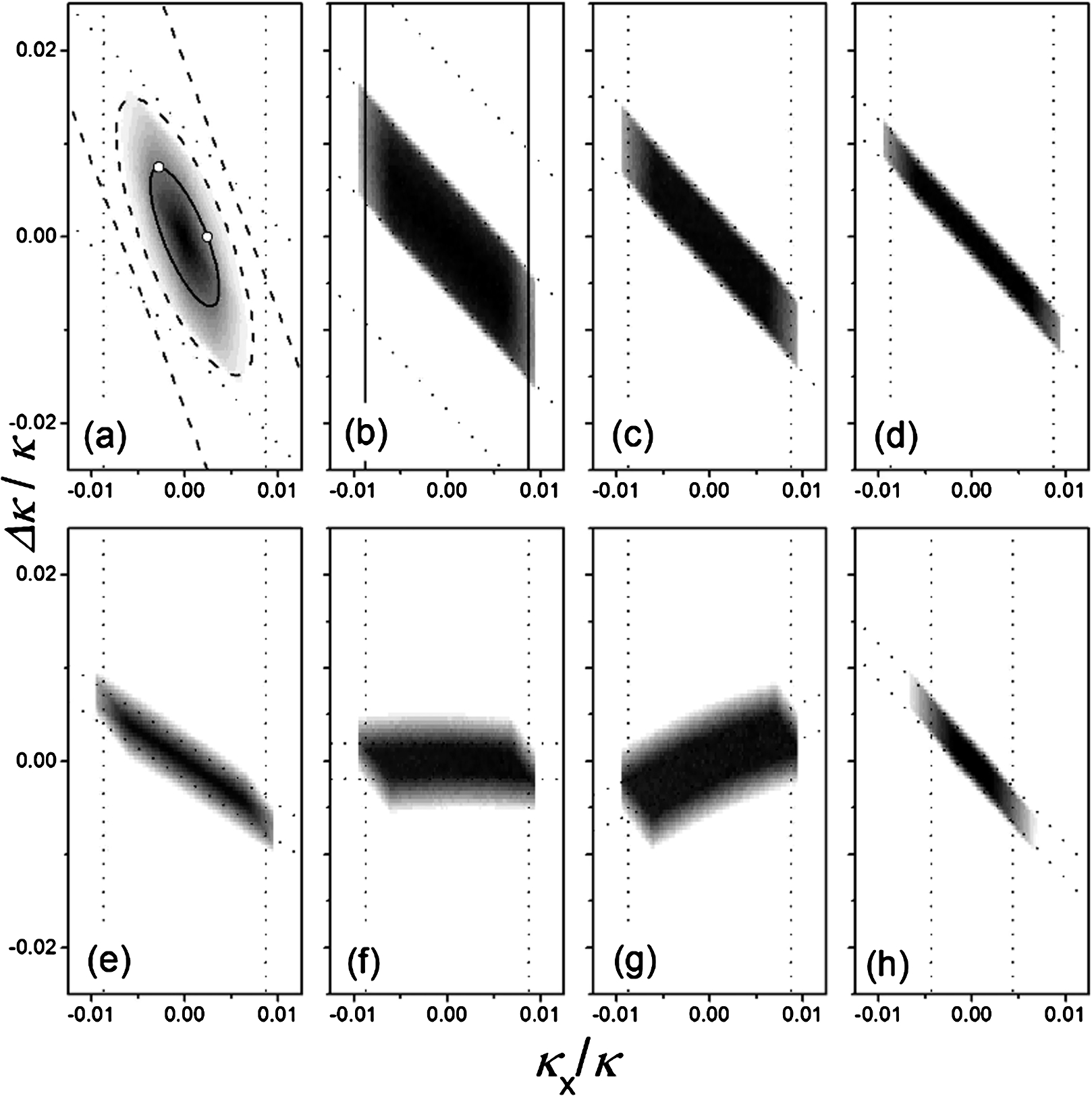
While the mathematics is clear, some of the conclusions may be surprising. To provide independent support for the accuracy of the mathematics, a series of McStas Monte Carlo computer simulations were conducted with the results presented in Fig. 11. These pictures show an effectively identical (i.e. the same A, B, C chosen here to be suitable for a high resolution PD) produced by widely different PS configurations. The simulated transmission over a 10 mm wide sample is plotted as a greyscale map of . The solid and dotted line elliptical contours represent the calculated and contours for Gaussian elements. The vertical dotted lines represent the limits imposed by while the pairs of sloping lines represent the limits imposed by and . All these simulations used Å, and a 15 cm wide source. The reactor face was modelled at 4 m from the source with the monochromator some distance further.
Figures 11(a)–(c) show configurations using Soller collimators and a flat mosaic monochromator. Figures 11(a) and 11(b) use values with ° and −60.51° respectively corresponding to a germanium (Ge533) monochromator. Note that reversing the sign of reverses the AD slope. This simply means that if is negative, decreasing increases the magnitude of and hence decreases the magnitude of κ. Figure 11(c) uses , i.e. Ge711, to produce an identical beam.
Figures 11(d) and 11(e) show configurations using a Radial Soller , a Soller collimator and a mosaic HFM with (Ge531) and (Ge 511) respectively.
McStas simulations of the sample position beam for different sets of instrument variables showing that a range of primary spectrometer arrangements and variable sets can deliver effectively identical beam characteristics. Figures 11(a)–(c) use a conventional PS with Soller collimators and a flat mosaic monochromator. Figures 11(d)–(e) use a PS with a Radial Soller–curved mosaic monochromator and Soller collimator. Figure 11(f) uses a PS with open beametubes and a curved mosaic monochromator. All examples deliver a Å beam and use . (a) ; (b) ; (c) ; (d) and ; (e) and ; (f) and using a 3.1 cm wide virtual source and a 2.4 cm wide slit just before the monochromator.
Figure 11(f) uses open beamtubes defined by slits at a virtual source and before the monochromator with a mosaic HFM. This arrangement gives results similar to that for the Radial Soller-flat monochromator-Soller arrangement discussed above but delivers rectangular profile and . The monochromator modelled used a Gaussian mosaic which means that does not have a fully rectangular transmission profile. Here , the virtual source is 0.031 m wide at 8.95 m from the monochromator and the slit before the monochromator is 0.0235 m wide. These values give element angular divergence HW a factor of smaller than the element FWHMs used for Fig. 11(d). This choice is to ensure that the rectangular profiles generated by the slits have the same angular variance as do the triangular profiles in Fig. 11(d). All curved monochromators were 15 cm wide and composed of 15 segments. All collimators and monochromators are assumed to have the same 100% peak transmission. The simulated flux at the sample was the same for the examples in Fig. 11(a)–(e) within 15% (as would be expected for equivalent ) but 135% higher for Fig. 11(f). The angular and average wave-vector variances were extracted from Fig. 11 data and the deduced standard deviations are presented in Table 1. The largest variation is 7.6% showing that is the same in effect for these very different PS configurations.
Standard deviations for wavevector spreads in Fig. 11
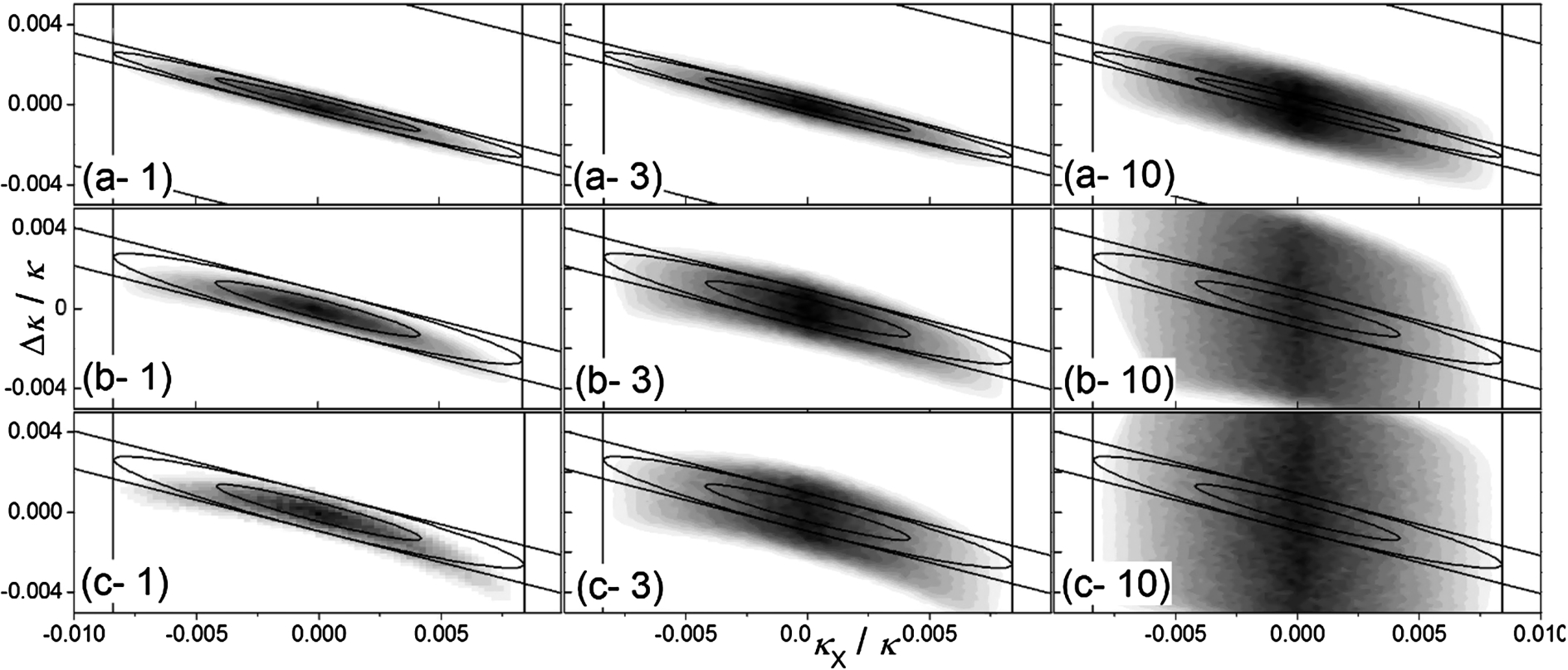
McStas simulations of the sample position beam using a PS with a Radial Soller-curved mosaic monochromator and Soller collimator with Å beam and . These examples show the effect of sample size (from left to right – 1 mm, 3 mm and 10 mm) with small . (a) and (Ge311); (b) and (PG002); (c) and (PG002).
It is possible to use even smaller values for to match here and some calculated examples for a Radial Soller-mosaic HFM-Soller arrangement are
(Ge311)
Pyrolytic Graphite PG002
PG002
This last example combines a negative with to produce an unchanged slope. Simulations of these configurations showed that matched those in Fig. 11 closely if the sample width was 1 mm but a 10 mm sample width showed a larger width and edges showing a noticeable curvature as illustrated in Fig. 12. These examples use small and large . Since the important quantity here is () it should be possible to equivalently use large and small but computer simulations showed that this approach led to even larger distortions. Figure 11 does demonstrate that an HFM can be used to greatly increase the range one can use effectively which may be very convenient for a number of practical reasons. Figure 12 shows that there is a limit to the theory where a check of spatial uniformity in the beam shows problems. Admittedly, Fig. 11 represents a rather extreme and very specialised beam type as required for a high resolution powder diffractometer to be used with a large range of sample scattering angle. The changes from very large in Fig. 11(a) to the very small in Fig. 12(b) and reversed small in Fig. 12(c) are also quite extreme. The origin of the aberrations shown in Fig. 12 is not clear. Reference [5] shows that decreasing in an open geometry PS increases the contributions from source width to the spatial and angular width of the sample beam spot size. Decreasing increases the contribution to the width from the source width while the contribution from monochromator width passes through a minimum at . The monochromators modelled in these simulations use segments on a flat base oriented to give angular displacements following a cylindrical curvature, so the monochromator curvature is not even truly cylindrical. It may be that a truly cylindrical curvature or perhaps some other curvature would reduce the aberrations seen here but such a study is beyond the scope of this work.
The exact equivalence of the PS AD for different choices of instrument variables only applies to beam elements with exactly Gaussian transmission functions. For triangular and rectangular distributions the “equivalence” is only approximate but Fig. 11 simulations show that it is “closely approximate”; perhaps better phrased as “usefully approximate”.
The fact that different choices of beam elements can deliver the same beam characteristics at the sample has academic interest but should also have practical use in overcoming the limitations inherent in available components. It is simple to continuously vary a slit width, vary monochromator Bragg angle or exchange collimators between discrete values. It is difficult to make high transmission Soller collimators with small divergence but simple to make a narrow slit (with high transmission). It is usually difficult to make large mosaic monochromators with high peak reflectivity and a given monochromator crystal may only be available with some particular mosaic. It is possible to interchange monochromators to change or or to adjust the relationship between λ and . It has been shown here that wave-vector spread can be adjusted by an slit width without changing . Using a curved HFM with smaller at a smaller can produce the same beam effect as a flat monochromator with larger at larger . Using slits to produce rectangular transmission profiles which increase intensity for a given resolution is simpler, cheaper and more controllable than using guides or reflecting Soller collimators. Background considerations may affect the choices but these are difficult to predict and very difficult to simulate accurately.
Most importantly, a given can be produced by different choices of primary spectrometer elements. Therefore, attempting to optimize an instrument design using the beam elements as variables must be hindered by the significant parameter covariance. This can be avoided by using a set of variables which describe the beam character, such as (u, , ). No doubt other variable choices could be made.
Adjusting the primary spectrometer to achieve a desired beam character
Section 6 showed that many different PS configurations can deliver equivalent beams. This section shows that a single PS design can deliver widely different beams as illustrated by . There are many ways of dealing with the choices available to deliver a given beam character but this section only discusses two. The first uses a PS with open beamtube and with a mosaic HFM curved to match the slopes of and . The second examines a PS using a HFM of small mosaic on a guide of rather large giving relatively large angular divergence in the incident beam.
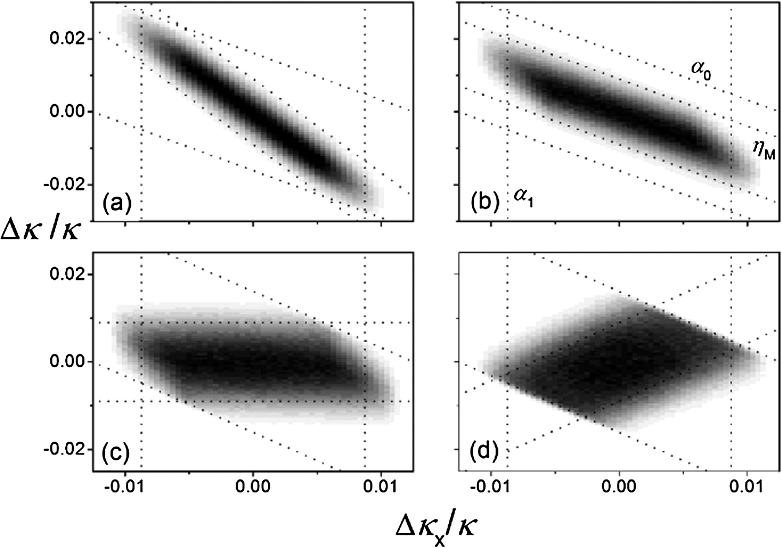
McStas simulations of for a PS with aligned & in various configurations. The superimposed lines show the expected full width contours for , and . Figure 13(a) shows for a conventional PS using Soller collimators and flat monochromator while Figs 13(b)–(h) show for a HFM virtual source PS using beamtube collimation. (a) . (b) . (c) . (d) . (e) . (f) . (g) . (h) .
Figure 13 shows McStas simulations of a PS using open beamtubes and a mosaic HFM as an independent confirmation of the calculations presented above. Figure 13(a) acts as a reference point and shows over a 10 mm width for a PS using Soller collimators and a flat mosaic monochromator with at Å (PG002 monochromator).
Figure 13(b) shows for a PS with . There is much to note in Fig. 13(b). Firstly, the open beamtubes lead to approximately rectangular profiles limited slightly by the Gaussian monochromator mosaic modelled. is achieved using cm and setting a rectangular profile of HW . is set by a slit of width 3.8 cm just before the monochromator with giving a rectangular HW . The rectangular profiles result in an slope which differs visibly from that in Fig. 13(a) as would correspond to a larger . Note that the value of limits the variation but that the Gaussian monochromator mosaic causes a rounding of the top of .
Figure 13(c) shows the effect of increasing the monochromator mosaic to (flattening the peak transmission of and increasing its average) while reducing to rectangular HW. Figure 13(d) shows the effect of reducing to . This clearly demonstrates that if a large enough monochromator mosaic is chosen, the width at the vertical axis of is effectively fully controlled by , i.e. by the virtual source slit width. Note that this is independent of the slope of .
Figures 13(e), (f) & (g) show that varying (to 4.0, 2.0 and 1.5 m) while keeping alters the slope of . Note that at each value of , must be adjusted to keep constant at and is adjusted according to Eq. (12) to maintain conventional full focussing. Note that the slope of can be varied and even reversed while keeping (and hence λ) fixed. Varying would alter the slope and width (by a factor) as well as changing the wavelength. The theory says that in this configuration with a large , (here controlled by the slit width ) should control the width. Figure 13(f) shows a significant extra broadening in for the 1 cm wide sample. This is not the case for smaller sample widths and thus, for “extreme” focussing conditions where becomes small the sample width may have to be reduced to reduce the wave-vector spread (corresponding to energy width in the scans). There may be circumstances where this spread is acceptable.
Figure 13(h) shows that (controlled using a slit before the monochromator) controls the overall width (and width) of . Here, . The intensities observed over a 1 cm width sample for Figs 13(a)–(h) are in the ratio . Notice that for the plots showing a change in the ratio with a corresponding change in the monochromator curvature (Figs 13(d), (e), (f) & (g)), a larger ratio results in larger sample flux.
Figure 13 shows that the behaviour of with rectangular transmission profiles closely follows that expected from the relations in Section 4. Adjusting the virtual source width changes the width measured parallel to the axis with no other effect. Adjusting using varies the calliper width parallel to the axis. Adjusting (while simultaneously varying to maintain and varying to maintain source to sample focussing) changes the slope of . At small ratios of , significant aberrations appear resulting in a broadening. This is not evident for a 1 mm wide sample beam but is apparent for the 10 mm wide beam shown here. Tests showed that the distortions observed here appear to be smaller at larger values of .
For a primary spectrometer situated on a guide source it is effectively impossible to vary so one must accept the slope supplied by the guide and set by . If the instrument is sited at the end of the guide, it may be possible to position a virtual source at the guide end and site the monochromator at some distance to exploit the flexibility offered by this arrangement. A purely numerical optimization study [14] found such an arrangement to be useful. For instruments on non-end guide positions, within the guide is set by the choice of λ, usually to a rather small value. In some cases, it may be possible to use interchangeable collimators between guide and monochromator to reduce the width of . By using a monochromator of fairly small mosaic one can control the slope by varying . A slit just after the monochromator can be used to control and thus the width of .
for HFM at the end of an guide with , Å at °. (a) Flat monochromator. (b) Focussed monochromator with . (c) “Over”-focussed monochromator with . (d) “Over”-focussed monochromator with showing reversed slope.
Figure 14 illustrates the effect of varying the HFM curvature on a long guide. The simulated and illustrated here uses a 3 cm wide guide at 2.36 Å (so ° or ) with a Ge111 monochromator with and °. With , with a rectangular profile. The monochromator has variable curvature with values in Fig. 14 of (a) Flat; (b) (Eq. (12) focussing); (c) and (d) . This figure illustrates very clearly that results from the superposition of , and . The relative intensities over a 1 cm wide sample are showing that the main effect of a HFM is to alter the slope with any intensity variation due to the changing overlap with . The reversal shown in Fig. 14(d) may be useful. For instruments on a guide, using the “zigzag” focussing arrangement for monochromator and sample scattering becomes difficult if using a small as the secondary spectrometer then collides with the guide shielding. Reversing the slope reverses the sample scattering sense needed to focus scans. It is likely that the increased intensity from focussing scans would outweigh any loss in sample position flux from this approach.
If working on a beamtube rather than a guide, one way to reverse the slope is to fix , choose a small and vary to rotate . One could set to set the axis parallel to the axis. Another way to achieve the same end would be to use a large with to set the axis parallel to the axis and then use a small and vary to rotate .
A modified primary spectrometer design
As described above, the character of the sample position beam can be visualised as an area, , in a 2D wavevector space bounded by an irregular hexagon where the transmission profile, , is the product of , and . The transmission is modulated by the angular transmission profiles of the PS collimators and monochromator mosaic. The key variables describing that region are its widths (both limiting and axis intercepts) and its slope.
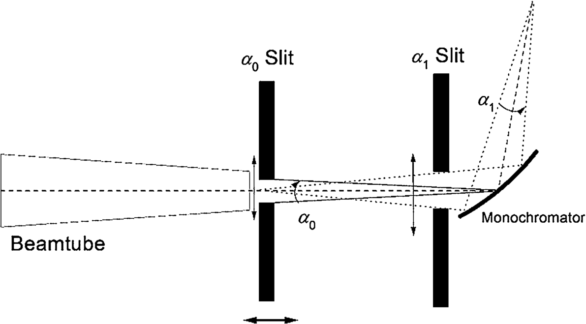
Instrument resolution and wavelength are commonly configured by exchanging PS Soller collimators and monochromator crystals. It would be useful to have a PS where the beam character could be varied to some desired form using only simple remotely controlled elements. Ideally, some simple calculations and remote adjustments would suffice to deliver some desired beam character with the maximum possible transmission. The PS design illustrated in Fig. 15 offers a way to achieve all this.
In the proposed design, the source is followed by a heavy slit (virtual source) with both variable slit width, , and variable position, , between the source and monochromator. A second heavy slit just before (or just after) the monochromator controls and hence (). The mosaic monochromator has variable curvature.
Schematic of novel primary spectrometer using open beamtubes, a horizontally curved mosaic monochromator, a variable width “virtual” source heavy slit with variable position between source and monochromator and a variable width heavy slit before the monochromator.
The choice of monochromator material is usually quite restricted by a number of factors; the availability of suitable large crystals, material absorption and coherence, crystal structure and spacing. Having chosen the monochromator material, the Bragg angle is then dictated by the desired wavelength.
Setting the monochromator radius of curvature to be (Eq. (12)) then aligns the axes of and and () and then have a similar effect in controlling the extent of at the axis. Monochromator mosaic often has a somewhat irregular profile but is usually modelled as having a Gaussian profile. Approximately rectangular profiles have been achieved using “onion peel” fabrication methods [12]. Since mosaic cannot be altered in situ, one way to maximise PS transmission would be to choose to be significantly larger than . The open beamtube here gives a rectangular transmission profile for and so the transmission profile of this combined function becomes approximately rectangular. For many monochromator materials, increasing reduces peak reflectivity but note that the important quantity here is so at “small” , great versatility may be possible even with a relatively small .
Varying can then be used to adjust the slope of . The distance from virtual source to monochromator, , controls the slope of and the choice of matches that to the slope of . In practice, the heavy slit could be mounted on rails in an open beamtube between the source and the monochromator, although the very heavy fixed shielding needed near the source may limit the range over which could be varied. Alternatively, a number of slits at discrete positions could be used.
The path between the monochromator and sample is also an open beamtube giving a rectangular transmission profile for and the value of sets () defining the limiting angular width of . The overall transmission profile inside is then close to rectangular maximising transmission at a given angular beam width.
The and slits could both be made very heavy and since both are inside the heavy out-of-pile beamtube or monochromator shielding this should effectively reduce background from fast neutrons and gamma rays from the source. Since the beamtubes and slits impose little restriction, much of the path length could be evacuated or filled with 4He gas to reduce air scattering.
This design offers great flexibility in choosing , the adjustments needed are simple and simply controlled remotely and the rectangular element profiles generated should maximise transmission. The key point illustrated here is that an understanding of the form of and its origin in PS elements allows the design of a PS with simply adjusted instrument parameters to achieve a wide range of beam character at the sample. The graphical approach offered by DDs or ADs facilitates that understanding. To best set up scans now only requires knowledge of the beam character needed to optimize instruments or measurements.
There are some potential challenges with this design although none seem too serious. Choosing a relatively large value for may reduce monochromator reflectivity if the crystal has significant incoherent scattering or absorption. It is difficult to calculate, model or simulate the background produced in a PS and an open geometry usually results in higher backgrounds but the very heavy slits and evacuated flight paths suggested here should mitigate that. If a large value is needed for , a large source width may be needed to fully illuminate sufficient monochromator width to permit large enough values for . Such wide beamtubes almost inevitably give high background and may lead to significant flux depression at reactor sources. Rectangular element transmission profiles can be expected to deliver measured scan peaks with non-Gaussian angular distributions which may complicate data analysis. While that may be aesthetically displeasing, since all but the simplest data is now routinely analysed by computer modelling, this is not a serious disadvantage as long as the profiles are accurately calculable or can at least be modelled.
Discussion and conclusion
This article presents a graphical view of the beam character transmitted by a conventional neutron primary spectrometer, with the discussion here restricted to the in-scattering-plane component of the beam, the most complex part of PS effects. Any full description must also include the existing description of the largely decoupled vertical divergence effects and possibly also of spatial effects. The graphical approach adopted (2D κ-space Acceptance Diagrams) treats the total sample position AD as a product or superposition of three ADs each associated with a single PS element. This approach permits a description and visualisation of the sample beam for a variety of collimator types and for curved monochromators. The mathematical formulae needed to accurately draw the pictures are presented in a way designed to clarify the effect of individual PS variables. Many sets of primary spectrometer variables can deliver the same beam character and equations are presented to calculate the allowed instrument variables for some chosen beam for several sets of constraints although other choices of constraints are possible. This flexibility in element choice can be used to make better technical choices and thus better cope with the limitations of available components. The form of presentation chosen here suggests a very flexible new PS design which delivers a maximised transmission. It would be interesting to see tests of these results on real instruments. Such tests of some limited set of the predictions here may be possible using flexible machines like TAS.
This work was originally done as part of an analytic derivation of optimal configurations for CW PDs but is presented separately because it has more general applicability. Apart from purely analytic approaches, there are other existing approaches to instrument design and improvement which have their own merits and drawbacks. For many years it was common to use the existing very complex formulae to calculate instrument resolution and to generate plots of scan profiles and beam character. The complexity of the formulations disguised the link between the PS variables and their effect on beams and scan profiles. Therefore, any exploration of the parameter space was necessarily time consuming and drawing firm general conclusions was difficult. More recently, the development of advanced MC computer simulation packages permitted the same sort of work with the advantage that other effects such as spatial beam variations and the effects of sample scattering could be considered. However, one central difficulty remained in the attempt to improve instruments. The existing equations and computer models could not unequivocally identify the performance trade-offs defined by the instruments and so the work had to proceed in an absence of defined quantitative performance measures in the form of numerical quality factors. Any attempt to deduce the performance trade-offs from a study of numerous calculations or simulations with a very large parameter space was dauntingly difficult, to say the least. Therefore, the optimization of instruments more complex than pinhole SANS has proved elusive.
At first glance, the study presented in this work probably appears quite dull with perhaps some minor academic interest. The work’s primary motivation is to facilitate the improvement of machines and the results presented here have already proved central in deducing optimized configurations for constant wavelength powder diffractometers [9,10] which demonstrate very exciting improvements. It seems clear that the approach developed in this paper would also allow the calculation of optimal element choices for SXDs and TAS (where the secondary spectrometer is an inverted primary spectrometer). For TAS two potential approaches suggest themselves. The first is to calculate formulae for scan profiles under a Gaussian approximation and then apply an undetermined multiplier method to maximise transmission at given resolution as done for CW PDs in [9]. This would probably be rather tedious but would provide a clear mathematical proof that the results were indeed optimal. A second, simpler approach would be to accept the conclusion in [6] that the TAS optimization requires matching the ADs of the “primary and secondary spectrometers” in a scan and apply the approach described here to choosing elements to achieve that matching. For TAS, one would make a choice of the reciprocal space volume to be sampled in each direction; thinking about how to make that choice should be instructive in itself.
It seems very likely that a Dumond Diagram approach would allow the optimization of Time-of-Flight (ToF) instruments. ToF sensitive area detectors can be assumed to be more or less universal on modern ToF machines, so the detector sees an intensity plot in a λ–θ space, i.e. a Dumond Diagram. Expressing the beam scattered by the sample as a DD based on a DD model of the beam incident on the sample should provide a relatively straightforward path to an optimization. Given that the majority of future sources for advanced neutron scattering are likely to be spallation rather than reactor sources and the logical development of predominantly TOF machines at such sources this may be among the most interesting avenue for future studies of instrument optimization.
The PS variable multiplicity discussed here means that there is significant parameter covariance in the description of beams. This means that any attempt to optimize neutron scattering instruments using the instrument parameters as the variables in a purely numerical approach, as is now being done using MC simulation packages, must somehow deal with this covariance. Choosing parameters which describe the beam character rather than just the beam elements can remove this covariance from the problem. Implementing this in existing software packages is likely to be very challenging.
One result from the present work which deserves emphasis is that the novel PS design described demonstrates a way to produce rectangular angular transmission profiles, , using open flightpaths without the need for special devices like guides or reflecting Soller collimators. Any such devices inevitably introduce transmission losses. Rectangular transmission profiles deliver the maximum transmission possible for a given beam angular variance thus improving instrument efficiency especially if no new losses are introduced.
The important assumption adopted here that the beam at the sample centre is representative of the whole beam appears to be valid over a wide range of parameter choices but seems to break down in some cases so perhaps some further work could seek an explanation and cure. Nowhere in this work is it assumed that the radiation considered is neutrons so the formalism may also be useful for X-Ray or electron scattering instruments if the instrument resolution is dominated by the beam elements. It is hoped that the formalism and the limited set of results and deductions presented here will provide a useful tool for better instrument design and better measurements.
Footnotes
Acknowledgements
LDC gratefully thanks Peter Willendrup who collaborated on some early MC simulations of some of the effects discussed here and Manh Duc Le for useful discussions.
References
1.
G.Caglioti, A.Paoletti and F.P.Ricci, Nucl. Instrum. Methods3 (1958), 223–228. doi:10.1016/0369-643X(58)90029-X.
B.Hamelin, Institut Laue Langevin annual report, 1996. Available at https://www.ill.eu/en/science-technology/neutron-technology-at-ill/optics/monochromator-crystals-group/monochromators/copper-crystal-mosaic/technique-onion-peel/.