





Abstract
The excessive radiation doses in the application of computed tomography (CT) technology pose a threat to the health of patients. However, applying a low radiation dose in CT can result in severe artifacts and noise in the captured images, thus affecting the diagnosis. Therefore, in this study, we investigate a dual residual convolution neural network (DRCNN) for low-dose CT (LDCT) imaging, whereby the CT images are reconstructed directly from the sinogram by integrating analytical domain transformations, thus reducing the loss of projection information. With this new framework, feature extraction is performed simultaneously on both the sinogram-domain sub-net and the image-domain sub-net, which utilize the residual shortcut networks and play a complementary role in suppressing the projection noise and reducing image error. This new DRCNN approach helps not only decrease the sinogram noise but also preserve significant structural information. The experimental results of simulated and real projection data demonstrate that our DRCNN achieve superior performance over other state-of-art methods in terms of visual inspection and quantitative metrics. For example, comparing with RED-CNN and DP-ResNet, the value of PSNR using our DRCNN is improved by nearly 3 dB and 1 dB, respectively.
Introduction
X-ray computed tomography (CT) imaging technology has been widely applied in various diagnostic and treatment tasks in modern medicine. Considering the increasing use of CT technology, the radiation hazards in CT can induce leukemia, cancers, and other diseases and are a major concern for the public [1]. In 1990, Naidich et al. [2] was first proposed the concept of low-dose CT (LDCT), and the dose level of LDCT is usually set as one-tenth of the regular dose CT (5–7mSv). Therefore, in view of above health concerns, the LDCT technology has attracted much attention in the field of CT imaging. In actual clinical applications, the most direct and effective strategy is to lower the tube current of the scanning process and consequently the number of photons received by the detector. However, directly reducing the current can severely degrade the quality of the images because the decaying photons induce a redundant quantum noise in the sinogram domain [3, 4]. To address this problem, many methods have been proposed to enhance the reconstructed CT image quality. These strategies can be broadly divided into three categories: sinogram restoration techniques, iterative reconstruction (IR) algorithms, and image post-processing techniques.
Before the application of analytical reconstruction algorithms, such as filtered back projection (FBP), sinogram restoration techniques are performed on the original data or logarithmically transformed data. The major advantage of these methods is that the projection data can be exploited more extensively, and the noise characteristics can be well characterized in the sinogram domain. In the past decades, some typical methods have been developed in the sinogram domain, including penalized weighted least-squares algorithms [5], anisotropic diffusion filtering [6], bilateral filtering [7], segmentation-based adaptive filtering [8], and structure adaptive sinogram filtering [9]. However, these sinogram restoration-based methods are often limited in practice, because the original CT projection data are not always accessible and typically have a low spatial resolution and/or newly generated artifacts.
The methods based on the IR algorithm are derived from the projection statistical data of the CT measurements and can improve the quality of image reconstruction more effectively than the analytical reconstruction algorithms. Recently, compressive sensing (CS) [10]-based constraints were used in statistical IR reconstruction to deal with cases of low dose, sparse view, and limited angle, such as image priors information-based approaches, including the total variation (TV) regularization and its variants [11–13], non-local means (NLM) [14, 15], tight wavelet frames [16], and dictionary learning [17, 18]. Although these methods perform satisfactorily in improving the image quality, they strongly depend on the form of the regularization function and the related settings of the parameters, thus limiting their practical applications.
Unlike sinogram restoration-based techniques and IR algorithm-based methods, image post-processing is an alternative technique to improve the image quality, as it does not depend on projection data and can directly process LDCT images. Based on the theory of CS, an adaptive K-SVD approach [19] has been proposed to reduce artifacts in CT images. Further, the block matching 3D (BM3D) [20, 21] method has proven to be efficient in various CT imaging fields. Recently, Green et al. [22] introduced a method utilizing the nearest-neighbors in-built high signal-to-noise ratio (SNR) patch database to replace noisy image patches. Hasan et al. [23] proposed a blind source separation (BSS)-based CT image reconstruction method using a multi-frame LDCT image sequence. These conventional image-domain post-processing methods can effectively improve the quality of a reconstructed image; however, the reconstructed images often have excessive smoothing or residual errors given that an accurate distribution of the image noise cannot be statistically determined.
In recent years, the convolution neural network (CNN) with its strong learning ability and outstanding performance has further promoted the development of CT imaging methods [24]. Deep learning (DL) techniques involve simulating the procedure of human information processing and efficiently learning advanced features from pixel-level data through a layered network framework [25]. Various DL-based denoising methods have been proposed, with promising experimental results. In [26], Han et al. combined the U-net model with residual learning to reduce the artifacts in sparse-view-reconstructed CT images. Jin et al. [27] proposed a deep convolutional network framework, combining FBP, U-net architecture, and residual shortcuts to preserve the image detail structure more effectively. Kang et al. [28] proposed a wavelet framelet-based deep residual network to suppress the noise in LDCT images. In [29], Chen et al., inspired by the idea behind the auto-encoder, proposed a residual encoder–decoder convolutional neural network (RED–CNN) to remove the noise induced during FBP reconstruction. Yang et al. [30] improved the quality of LDCT images by constructing 2D and 3D residual CNN networks, and found that the proposed models can achieve better performance in terms of edge feature preservation. More recently, Lee et al. [31] proposed a deep network model for complementing sparsely sampled sinograms to reduce the noise in LDCT images. Yuan et al. [32] proposed a residual U-net architecture-based mixed DL method, which combines sinogram interpolation and image denoising to improve the image quality. Although the results were promising, there remained undesirable errors between the processed sinograms and the normal dose sinograms, and these errors were amplified during the image reconstruction process, resulting in blurred reconstructed image textures and loss of structural details.
Despite the promising results obtained in the case of employing either the sinogram domain or the image domain for LDCT imaging, the potential of combining the sinogram and image domains to improved image quality has not been fully investigated. For example, Huang et al. [33] designed a two-stage residual CNN model to reduce noise and retain texture structure information on LDCT images. Meng et al. [34] construct a semi-supervised learned sinogram restoration network to improve the quality of LDCT, which is comprised of supervised sub-network and unsupervised sub-network. Therefore, we proposed a dual residual convolution neural network (DRCNN), which can improve the entire imaging process by converting the noisy sinogram to a denoised CT image. The DRCNN is composed of three main units: a sinogram-domain sub-net, an FBP module, and an image-domain sub-net. Figure 1 shows the proposed neural network-based imaging strategy. Specifically, the two cascaded blocks in the proposed network are linked by an FBP layer, which decodes the sinogram into CT images to avoid the overfitting problem. Moreover, we simultaneously train the sinogram-domain and image-domain sub-nets instead of independently training them, to reduce the calculation time.
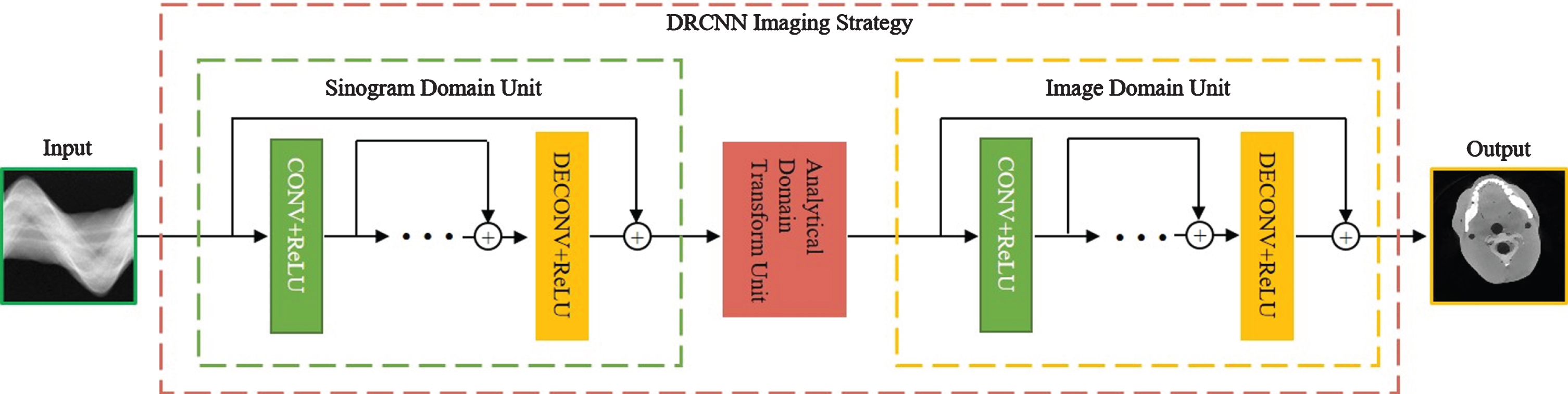
Proposed DRCNN imaging strategy.
The rest of this paper is organized as follows. Section 2 presents the detailed network model structure and training method. Section 3 describes the data specification and experimental results. Finally, discussions and conclusions are presented in Section 4.
Noise reduction model
The pipeline of the DRCNN has three main units: the first unit, i.e., the sinogram-domain sub-net, is used to reduce the noise and complete the sinograms. The middle unit is responsible for transforming the processed sinograms into LDCT images. The last unit, i.e., the image-domain sub-net, is designed to further reduce the noise and artifacts that remain in the LDCT images.
Assuming that x ∈ RM×N represents an original sinogram of the LDCT and y ∈ RM×N its corresponding normal-dose reference sinogram, the objective of the denoising process in the sinogram-domain sub-net is to learn a function G1 that maps the original sinogram x to the normal dose sinogram y:
Typically, the fully connected layers are utilized to map elements from the sinogram unit to the CT image unit [35]. This process increases the number of parameters and therefore the computational complexity. To solve this issue, we adopt the FBP transform layer instead of fully connected layers to decode the output of the sinogram-domain sub-net into a CT image with low signal-to-noise ratio, as follows:
The two main types of noises induced during the LDCT imaging process are the electronic background noise and the X-ray photon statistical noise, which approximately obey the Gaussian and Poisson distributions, respectively [36]. Consequently, in the entire reconstruction process, the noise model is complicated and non-uniformly distributed, and it is difficult to solve this problem using conventional methods. For deep neural network-based methods, the uncertainty of a noise model can be ignored owing to the capability of the deep neural network itself in learning high-level features and representing the data distribution [37]. Therefore, the proposed DRCNN model is designed on the basis of the effectiveness of the residual structure for preserving details in low-contrast regions, and is an effective strategy to reduce the sinogram noise and extract image features.
The architecture of the proposed DRCNN network comprises three parts, in which the residual shortcuts are utilized as the basic network architecture because they can effectively restore the meticulous details in the targets. Specifically, the first part is the sinogram-domain sub-net used to process the projection data. The projection data returned by this sub-net can be considered approximately clean. Subsequently, the processed projection data are inputted to the FBP reconstruction step to reconstruct the LDCT images. The last part is the image-domain unit, which repairs the reconstructed LDCT images, the results of which can be considered an approximation of the normal-dose CT (NDCT) images.
Residual structure network
The performance of a network can be improved by stacking more layers; however, in the general form of the network shown in Fig. 2(a), the convolution neural-based networks only have connections between adjacent layers, and as the depth of the network increases, the training loss will increase. To solve this problem, He et al. [38] proposed a residual connection structure to add a simple identity mapping between the input and the output of a set of layers. The residual connection brings two advantages. First, the explosion/vanishing of the gradient is avoided. Second, the high-resolution structural and contrast details are preserved, thus significantly promoting the network performance. Since then, researchers have added residual learning to CNNs for denoising LDCT images, with interesting results [39–42].
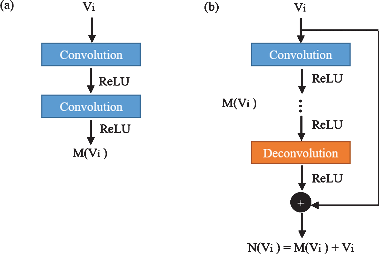
Forms of general and residual connection networks: (a) universal network, and (b) residual structure network.
Unlike the general network shown in Fig. 2(a), a basic residual structure network is composed of multiple stacked convolutional layers and deconvolutional layers, as shown in Fig. 2(b). We applied three residual connection modules and two residual connection modules in the sinogram-domain sub-net and image-domain sub-net, respectively, to preserve more detailed information (as illustrated in Fig. 3).
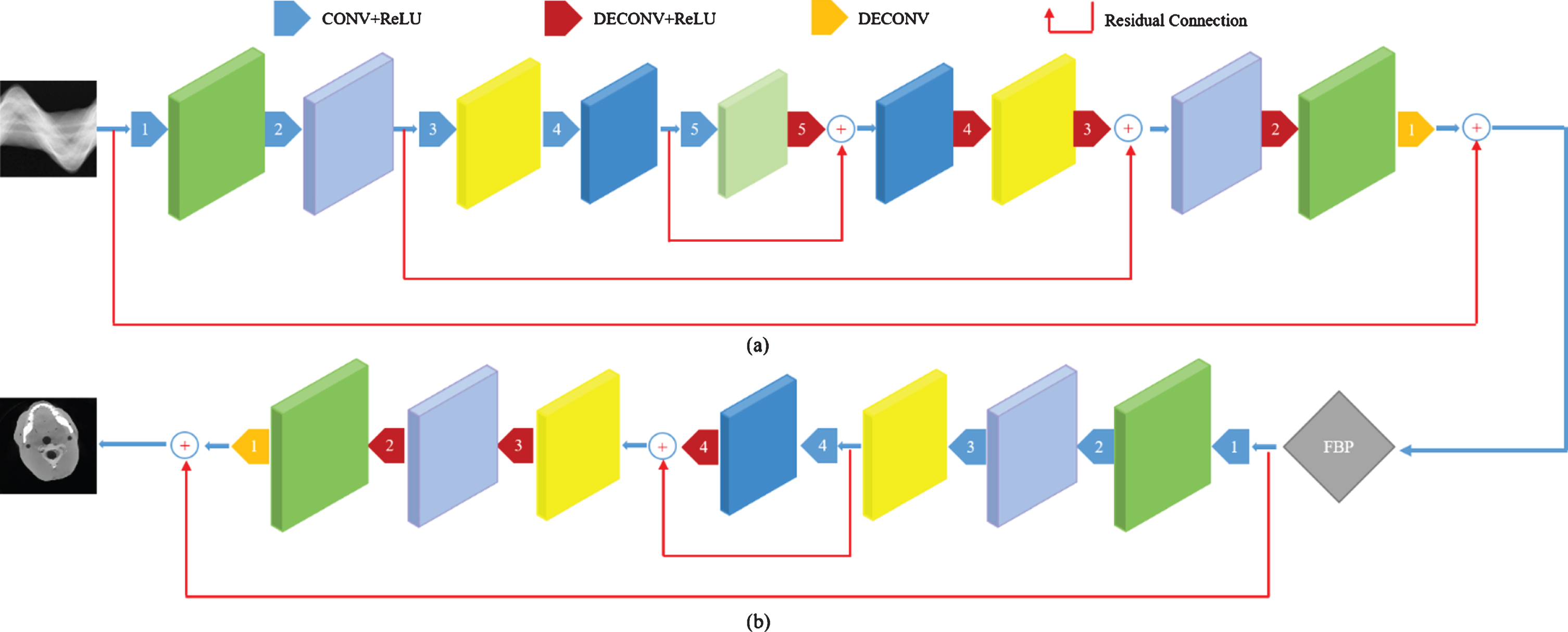
Overall architecture of the DRCNN network: (a) sinogram-domain sub-net, (b) image-domain sub-net.
Under the premise of the mapping function (1), the objective of the trainable layers in the sinogram-domain sub-net (shown in Fig. 3(a)) based on the residual structure network is to predict the noise component in the sinogram of the LDCT. Through the normal-dose sinogram used in the training process, the sinogram-domain sub-net transforms the LDCT sinogram into a noise-reduced output sinogram.
We construct our sinogram-domain sub-net based on the RED–CNN, which is developed to effectively remove the widespread and complex noise existing in LDCT sinograms. The sinogram-domain sub-net consists of five convolution layers and five deconvolution layers, and all the trainable layers have small convolution kernels with a size of 5×5 pixels. The number of kernels except for the final layer is 128 for all layers in the sinogram domain sub-net. Each layer except for the last one is followed by rectified linear units (ReLUs) [43], which help prevent the gradient from disappearing and help accelerate the network convergence. The final layer is used to subtract the noise component from the raw data to reconstruct the sinogram. To prevent the vanishing of the sinogram edges after each convolution, we apply the zero-padding operation to the sinogram-domain sub-net to maintain the sinogram size. Compared with the CT projection measurement, the magnitude of the projection noise is relatively small; therefore, we initialize the weights in each convolution layer to a normal distribution with a standard deviation of 0.01. As shown in Fig. 3(a), we use three basic residual structure networks to reduce the pixel loss induced during each convolution. Specifically, the input sinogram and the input of the layers 3 and 5 were connected to the output of layers 10, 8, and 6, respectively.
Image-domain sub-net architecture
In the case of residual faint noise in the denoised sinogram, the LDCT images reconstructed by the FBP were degraded because of the sensitivity of the reconstruction process to the errors. Therefore, we constructed the residual structure network-based image-domain sub-net to predict the undesirable components of the noise and artifacts in the LDCT images and thereby improve the image quality. The proposed image-domain sub-net (depicted in Fig. 3(b)) reduces the noise by learning the end-to-end mapping from the noisy LDCT image (reconstructed by the FBP) to its corresponding noise-free NDCT image. The sizes of the input and output images are both 512×512 pixels.
Unlike the sinogram-domain sub-net, four convolutional layers and four deconvolution layers are used in the image-domain sub-net, which help reduce the image noise while preserving more structural features (more detailed information regarding model determination is provided in Section 3). The convolutional layer acts as a feature extractor in the CT image domain, which preserves the primary components of the image. The corresponding deconvolutional layers are then merged to restore the details of the image contents. Particularly, to extract image features more effectively, the patch size is set to 48×48. The consecutive eight trainable layers have filters of size 5×5 pixels, and the convolution stride is set to 1. The number of kernels is 128 in all the convolutional layers except in the last one, where the number of kernels is 1, and each layer except for the final layer is followed by ReLUs. The last layer of the image-domain sub-net is a single convolution layer, which is used to predict the noise components of the multiple channels from the previous layers. Subsequently, the noise components can be removed from the LDCT images to return the denoised images. Furthermore, to avoid feature blurring during the down-sampling operation, no pooling layer is used in the proposed network model. As shown in Fig. 3(b), the image-domain sub-net contains two basic residual structure networks. The input reconstructed LDCT image and the input of layer 4 are connected to the outputs of layers 8 and 5, respectively.
Objective function and network training
Different objective functions represent different penalizing mechanisms while generating a learned mapping. The mean square error (MSE) is widely used as an objective optimization function in low-level image processing tasks such as image restoration and image enhancement. Inspired by the ability of MSE in calculating the intensity difference between the output pixels and the ground truth images, it has been used in many low-dose CT noise reduction methods. In our work, we exploit the MSE between the denoised sinogram/image and the real sinogram/image as an objective function to ensure that the noise can be removed more accurately. The objective function of the proposed DRCNN model is composed of two terms:
Considering the good noise removal ability of the TV regularization term, in this study, the TV loss is integrated into the overall optimization function to further optimize the proposed DRCNN model. Reducing the TV loss can help decrease the difference between the adjacent pixel values in the LDCT images. The TV regularization term can reveal the sparsity in gradient magnitude images. The TV of the final output image
The network architecture controls its inherent presentation capability. In general, the deeper the model, the higher is its presentation capability. The proposed DRCNN is an end-to-end system based on multiple residual structures that map the original sinograms to the reconstructed CT images. Once the network architecture is successfully configured, the parameters of the network can be learned by optimizing the total loss function (6) using the FBP module [45], which has the ability to back propagate the errors from the image to the sinogram. During training, the parameters λ1 and λ2 are set to 1 and 100, respectively, and the weights of the TV loss are set to 0.5. To further improve the network performance, we train the DRCNN model for 50k iterations both in the simulated and real data experiments using the adaptive momentum estimator (Adam) optimizer [46], which is a gradient-based optimizer that considers first-order and second-order moment estimations of a gradient. The hyper-parameters for the Adam optimizer are set as follows: the initial learning rate is set to 0.0001 without any weight decay or dropout, the first momentum is set to 0.9, the second momentum is set to 0.999, and ɛ is 10–8, the same setting as that in the original paper. In the two experiments on the simulated and real data, the parameter settings of the DRCNN are the same. In total, 30.752 million parameters of the DRCNN should be learned during training. All the training and testing tasks are performed on the TensorFlow DL framework with a single GPU (NVIDIA TITAN V, 12 GB of memory).
Data preparation
Both the simulated and real data are utilized to verify the performance of the DRCNN. The experimental objective with the simulated data is to improve the effectiveness of the DRCNN for LDCT images. The noise intensities of the different settings are used to assess the robustness of the DRCNN. The experiments on the real data further prove that the DRCNN has clinical application prospects.
Simulated data
The normal-dose dataset includes 3589 NDCT images of 512×512 pixels per image of 12 patients (denoted with patient #1 to #12) collected from a local hospital [47], including images of different parts of the patient’s body for diversity (head and abdomen). And we classified 12 patients into a training group (patient #1 to patient #10) with 2990 NDCT images as a simulation training dataset and a testing group (patient #11 and patient #12) with 599 NDCT images as a simulation testing dataset. The corresponding LDCT image dataset was generated by adding the Poisson–Gaussian mixed noise to the sinograms simulated from the normal-dose images. Experiments on different phantoms have proved that Poisson-Gaussian mixed noise is closest to the real noise in LDCT images [36, 48]. In this case, the simulated images are more visually similar to the real LDCT images. The specific noise model can be expressed as,
In this experiment, the intensity and complexity of the noise are constrained by revising σ2 and N0, respectively. The difficulty in eliminating the noise varies with the intensity and complexity of the noise. Totally, three groups of simulated images with different noise levels are used for comparison. Table 2 lists the Poisson and Gaussian noise-related settings.
Comparative experiments on DRCNN versions
Because the continuous CT images are similar in terms of visual characteristics, the images in the simulation dataset are randomly selected to further enhance the ability of the DRCNN model in observing new images. Since DRCNN is an end-to-end system, we selected 887 normal-dose CT images randomly and non-continuously from the simulation training dataset, and produced 887 pairs normal-dose and corresponding low-dose sinogram images, which were used as the label and the data during the DRCNN training process. Similarly, we produced the simulation testing dataset composed of 196 low-dose sinogram images for testing the DRCNN model.
To further evaluate the potential of the DRCNN in an actual CT system, in this experiment, we selected the CDP (Chengdu Dosimetric Phantom) [49] radiological anthropomorphic human head model as the scanning object to study its clinical application prospects. The shape of the phantom likes the human head, and the equivalent error between the attenuation coefficient of the material used and the attenuation coefficient of real tissues or organs should not exceed 5%. The projection data are obtained by cone-beam scanning. In the normal and low-dose scanning experiments, the X-ray tube voltage both are set to 120 kVp, and the tube current is set to 109.02 mAs and 38.93 mAs, respectively. In addition, the distance between the X-ray source and the axis of rotation is 483.414 mm, the distance from the X-ray source to the detector is set to 796.494 mm, and the number of probes and the probe dimension are set to 1437 and 0.296 mm, respectively. The ray source model of the CT scanning system used in the experiment is Thales Hawkeye-130, and the flat-panel detector used is Varian 4030E. In the real data experiment, a total of 2000 pairs of normal-low dose phantom slice sinograms of 512×512 were collected as the real dataset. And we used the first 1200 pairs sinogram images as the real training dataset and the last 200 pairs sinogram images as the real testing dataset to train and test the DRCNN, respectively. In addition, in the data pre-processing process, the value range of all 512×512 sinograms is normalized to [0, 1]. Table 2 lists the specific scan parameters for the normal and low doses.
Comparison schemes
In our experiments, the images are reconstructed from the following six algorithms for comparison to assess the proposed DRCNN more objectively and accurately: LDCT image reconstruction algorithm based on the conventional FBP (expressed as LDCT), the IR algorithm with total variation (TV) regularization (expressed as TV), the BM3D; which represents the conventional image-domain denoising method, the DnCNN [50], the RED–CNN based on DL representing the state-of-the-art denoised methods, and the DRCNN method. The parameters of the TV, BM3D, DnCNN, and RED–CNN are set in accordance with the settings reported in the original papers and retrained or fine-tuned on the available LDCT images.
Quantitative evaluation criteria
To evaluate the potential improvement in the DRCNN model, we select four quantitative metrics to estimate the quality of the reconstructed images compared with the ground truth images, including the root-mean-square error (RMSE), structural similarity index measure (SSIM), peak signal-to-noise ratio (PSNR), and normalized mean absolute distance (NMAD). The three metrics (RMSE, PSNR, and NMAD) measure the absolute errors of the reconstructed images. Specifically, the higher the PSNR, the higher the image quality. Lower values of the NMAD and RMSE indicate small differences between the reconstructed results and the ideal image. The SSIM expresses the structural information in the reconstructed images. An SSIM value close to 1 indicates an exact theoretical reconstruction.
Model determination
We completed five sets of comparative experiments to validate the method described in Section II: NoTV, DRCNN-1, DRCNN-2, DRCNN-3, and DRCNN-4, respectively. NoTV represents that the TV regularization model is not applied in the proposed method. It only improves the performance of the network model by optimizing the losses in the sinogram and image domains. DRCNN-1 to DRCNN-3 represent three various network structures different from the proposed method and DRCNN-4 represents the complete process of the proposed DRCNN. And the specific network model structures and total training parameters of the 4 DRCNNs are listed in Table 1. Three different sets of noise intensities are simulated by the back-projection algorithm to demonstrate the advantages of the proposed architecture. Note that, based on the numerical results, only the middle group is most similar to the intensity of the real LDCT projection data acquisition process. Table 2 lists the numerical results of the representative slice, with the best results highlighted in bold.
The differences between of the 4 DRCNNs
The differences between of the 4 DRCNNs
Evidently, the quantitative results generated by the other four groups of network models with the application of the TV regularization term are better than those generated by the NoTV. This verifies that the TV regularization model is effective in preserving details and reducing noise. Furthermore, compared with the other three methods that also utilize the TV regularization model, DRCNN-4 further improves the quality of the reconstructed images, which reflects the necessity of using five convolution–deconvolution pairs in the sinogram-domain sub-net and four convolution–deconvolution pairs in the image-domain sub-net. We find that all the methods work well when a Poisson–Gaussian mixed noise with σ2 = 25 and N0 = 10000 is added.
Figure 4 shows the visual denoised results of the representative slices. The green rectangle, in (a) NDCT, represents the region of interest (ROI). The NoTV method loses image details as shown in the ROI of Fig. 4(c). Moreover, as shown in Figs. 4(d)–(f), there remains residual noise that need to be removed, and there are unclear image details as indicated by the orange arrow. By contrast, the DRCNN-4 is more accurate to the ground truth in terms of the contrast and luminance.
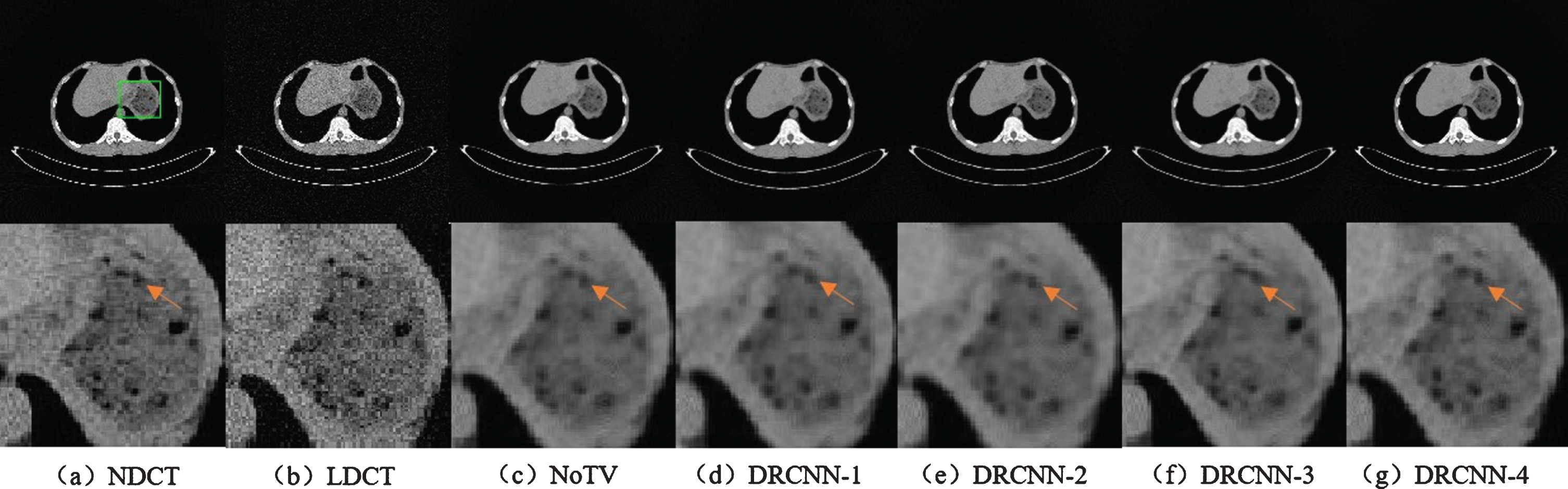
Noise reduction results of the methods involved. Group with a Poisson noise N0 = 104 and Gaussian noise with σ= 25 is added to the displayed LDCT image. The green rectangle in (a) represents the enlarged area.
Simulated data results
To evaluate the potential noise reduction capabilities of the compared methods and the DRCNN, two representative slices selected from the simulation testing dataset and the corresponding enlarged ROIs are shown in Figs. 5, 6, respectively.
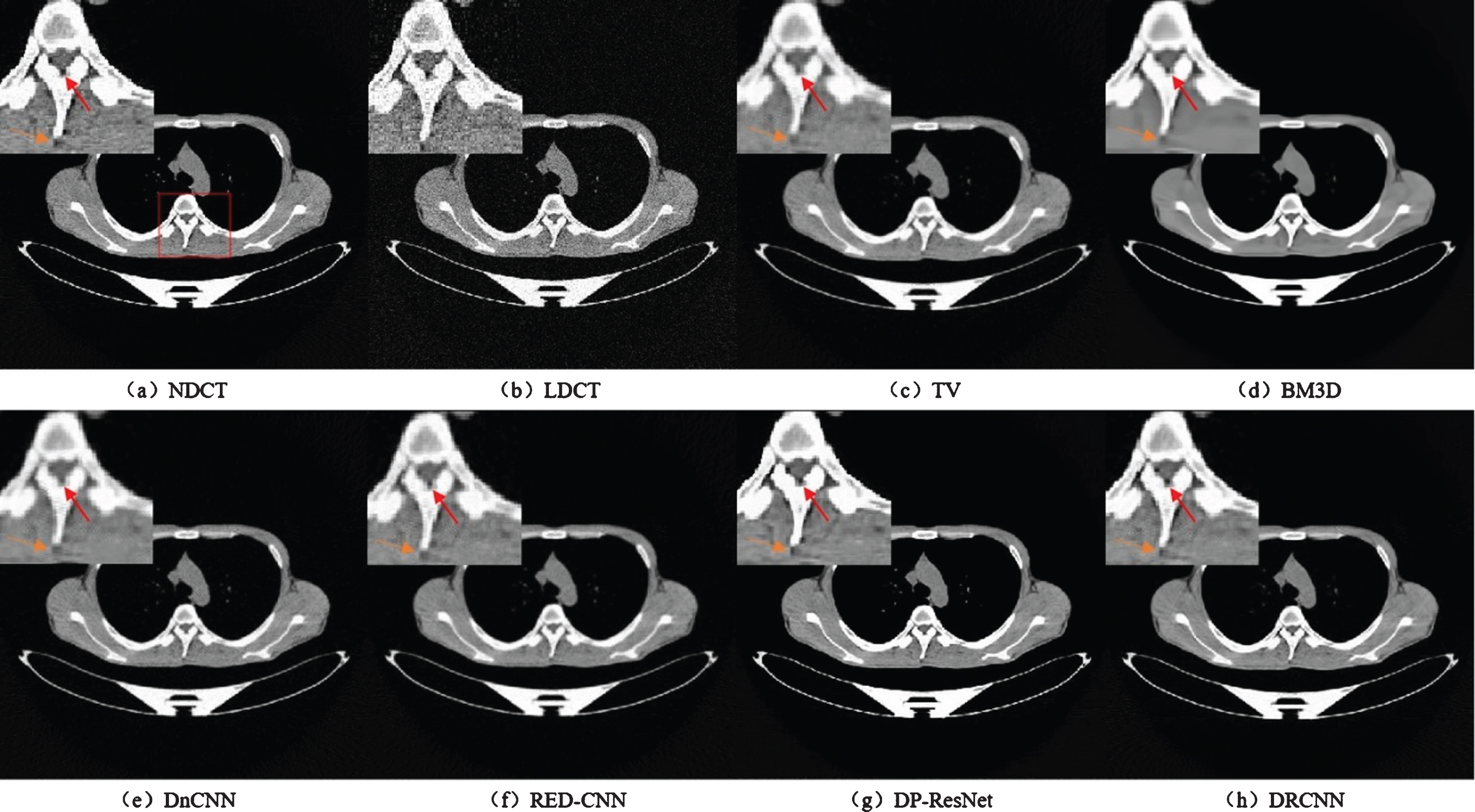
Results of the abdominal slice obtained using different methods. The red rectangle in (a) represents the enlarged area.
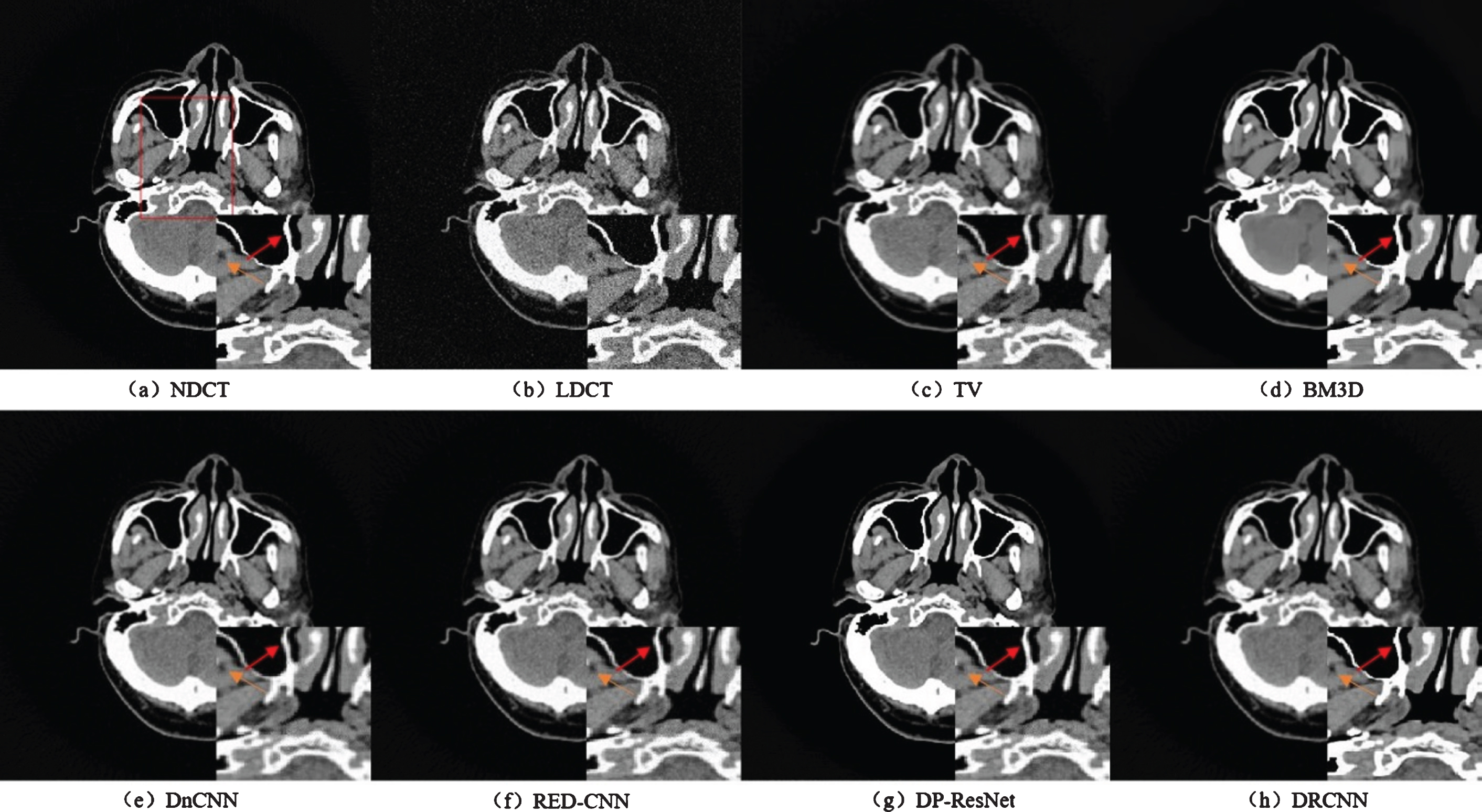
Results of the head slice obtained using different methods. The red rectangle in (a) represents the enlarged area.
Figure 5 shows the results reconstructed from the abdominal slice using the different schemes. Figure 5(b) shows that the image reconstructed using the classical FBP algorithm has high image noise and streaking artifacts. The iteration-type TV regularization model yields an improved image reconstruction quality with an effective suppression of the noise; however, some important small structures in the image are lost, as shown in the enlarged region of Fig. 5(c). Overall, the enhanced results of the classical BM3D method have high contrast in visual effects and preserve more structural information than the TV method; however, the denoised image is over-smoothed, leading to loss of critical details, which can significantly affect the diagnosis. As indicated by the orange arrow in the enlarged region of Fig. 5(d). Although the DL-based DnCNN and RED–CNN perform well in terms of noise reduction, the obtained images still exhibit over-smoothing characteristics, resulting in blurred image details, as indicated by the red and orange arrows in the ROIs shown in Figs. 5(e), 5(f). And we observed the image reconstructed from the DP-ResNet had blurred image details, as shown by the red and orange arrows in enlarged region in Fig. 5(g). By comparing the noise reduction results shown in Fig. 5, we find that the proposed DRCNN outperforms the compared methods in terms of the noise artifact suppression and soft tissue feature preservation, as depicted in Fig. 5(h).
Figure 6 shows the results of the head image. Like the image shown in Fig. 5(b), the simulated LDCT image is significantly deteriorated, and many details cannot be identified in Fig. 6(b). The TV algorithm cannot restore the image well, and the spatial resolution is also poor, as shown in the ROI of Fig. 6(c). From the results shown in Fig. 6(d), we find that, although the BM3D removes most of the noise, some texture information is lost, as indicated by the orange arrow in the enlarged region. The DnCNN and RED–CNN suppress the noise effectively and preserve most of the image details during denoising; however, undesired artifacts are induced near the bones, as indicated by the red arrow in the ROIs of Figs. 6(e), 6(f). According to the red and orange arrows in the magnified area of ROIs in Fig. 6(g), it can be clearly found that the reconstruction result obtained using DP-ResNet method has low-contrast tissue details. The DRCNN, as shown in Fig. 6(h), best preserves the linear high-attenuation structure of the head, which likely represents contrast-enhanced blood vessels. The proposed method better delineates the edges of the different tissues and preserves the critical information.
In addition to the evaluation on visual inspection, the denoising results are estimated using quantitative metrics, namely the PSNR, SSIM, RMSE, and NMAD. Table 3 lists the four quantitative indexes measurement results, with each quantitative metric score in terms of the measured mean values and their standard deviation of all the 196 images in the simulation testing dataset. The performance metrics of the TV and BM3D are inferior to those of the DnCNN, RED–CNN and DP-ResNet. This can be attributed to the strong feature extraction and learning capabilities of deep neural networks. Evidently, the DRCNN method is superior to the other neural network-based methods in terms of the numerical results. The above quantitative results are consistent with the visual effects shown in Figs. 5, 6.
Quantitative results (mean±std) of different methods for all 196 test images
Meanwhile, we used T test to analyze the statistical difference of the four evaluation indexes between DRCNN and other methods, and their P-value are calculated and presented in the Table 4. We can clearly observe that the P values obtained by LDCT, TV, BM3D, DnCNN or RED-CNN are much less than 0.01, which indicates that the statistical effect of DRCNN is much better than these five methods. Compared with DP-ResNet, totally four P value of four indicators between DRCNN and DP-ResNet were less than 0.01 except for RMSE, which proves that DRCNN is not significantly different from DP-ResNet on RMSE in the statistical level.
The T-test is performed on the data of the PSNR, SSIM, RMSE, NMAD data between DRCNN and other methods. P value of each set of data is given in the table
The DRCNN model is assessed using real scan projection data collected from the CT scans of the human head phantom. Figure 7 shows the representative slice results and the corresponding enlarged ROIs. The LDCT image shown in Fig. 7(b) contains significant noise. Although the TV method yields a good noise reduction performance, the image exhibits blurring interference, as shown in the enlarged areas of Fig. 7(c). As indicated by the red circles in the ROI of Fig. 7(d), the BM3D method loses some image details, which may affect the diagnosis. Although the performances of the DnCNN and RED–CNN are comparable to that of our method, we find that the low-contrast structure is smoothened in the enlarged areas in Figs. 7(e), 7(f), respectively. In Fig. 7(g), the results of DP-ResNet lost image details in tissue regions, as shown by the red arrows in the enlarged areas. Moreover, from the illustrations shown in Fig. 7(h), we note that the proposed DRCNN exhibits a superior performance both in terms of noise reduction and structure preservation.
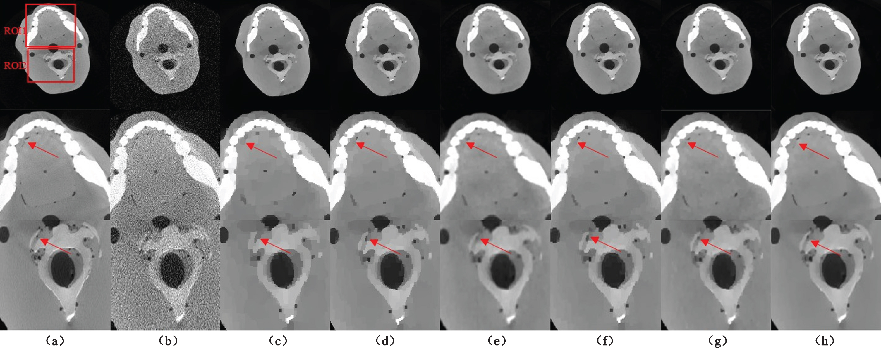
Head phantom reconstruction results obtained using (a) NDCT, (b) LDCT, (c) TV, (d) BM3D, (e) DnCNN, (f) RED–CNN, (g) DP-ResNet, (h) DRCNN methods.
To further demonstrate the merits of the DRCNN, the absolute difference images relative to the routine dose CT image are shown in Fig. 8. In the difference images, the darker the observed color, the lower the error. Clearly, the image obtained using the DRCNN has the lowest deviation from the original image, preserving most of the image details and largely reducing the noise and artifacts.
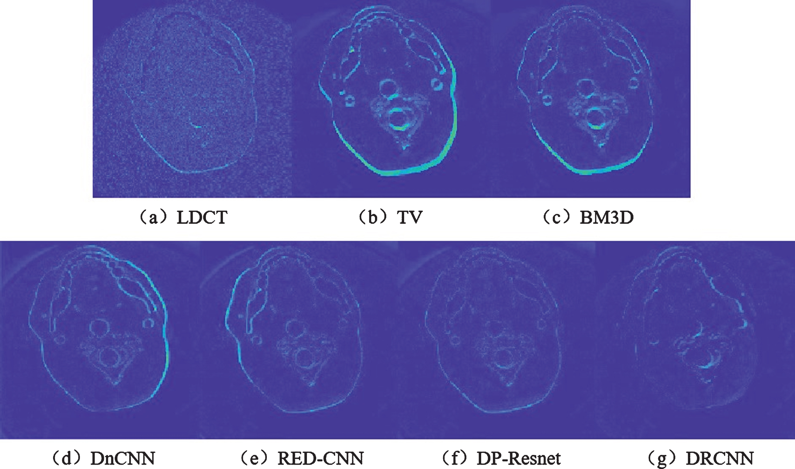
Absolute difference images obtained by different methods corresponding to the reference image.
For a quantitative evaluation, two ROIs are selected, as indicated by the red rectangle in Fig. 7(a). Figure 9 shows the quantitative measurements scores of the two ROIs. The quantitative comparative results represented in the form of bar graphs are consistent with the visual effect results shown in Fig. 7. The DRCNN yields the lowest RMSE/NMAD and highest PSNR/SSIM for both the ROIs.
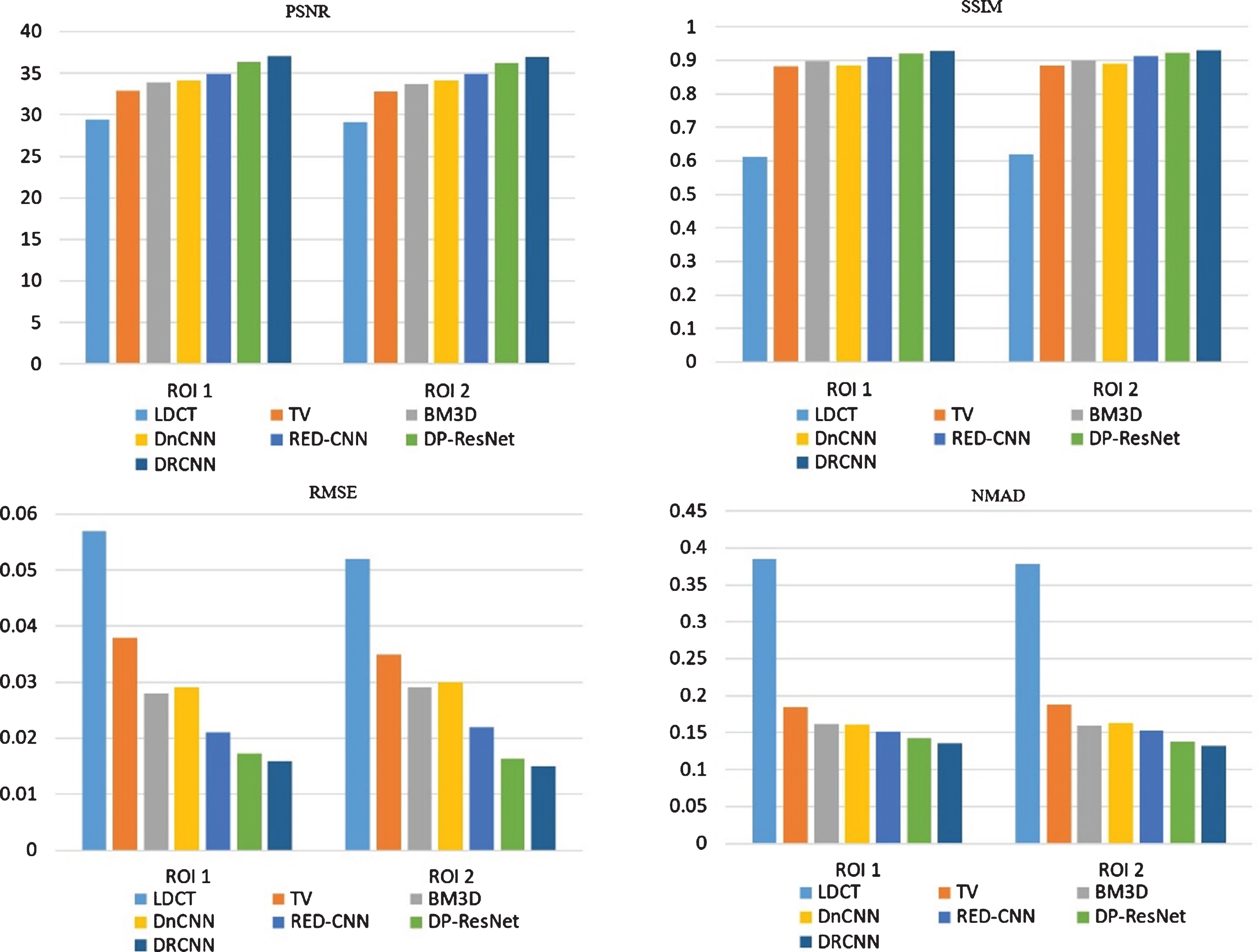
Quantitative performance comparison between the six methods over the two ROIs marked in Fig. 7(a).
The low network model efficiency is a major problem in DL. In this part, the network parameters of the DRCNN model are tested, including the number of filters and the weight values of the TV loss. The parameter analysis is carried out by varying the one to be explored while keeping the others constant. The data used for the parameter evaluation are randomly selected from the training data of the simulated datasets.
Filter number setting
In deep neural networks, a reasonable number of filters is beneficial for improving the training stability and data feature extraction capability of the network. We test the convergence performance of the network by varying the filter numbers in the sinogram-domain and image-domain sub-nets, with the other parameters fixed. Given that a higher number of filters is conducive for extracting the data features, we perform four groups of comparison trials, in which the numbers of filters in the sinogram-domain and image-domain sub-nets are set to 96 and 96 (as group one), 96 and 128 (as group two), 128 and 96 (as group three), and 128 and 128 (as group four), respectively. As shown in the training loss function curve in Fig. 10, the gains of the convergence speed of the four groups gradually decrease. The third group achieves the lowest loss value, although this phenomenon is not evident with increasing number of iterations. To balance the network performance and the computational complexity, the numbers of filters in the sinogram-domain and image-domain sub-nets are set to 128 and 96, respectively, in the DRCNN model.
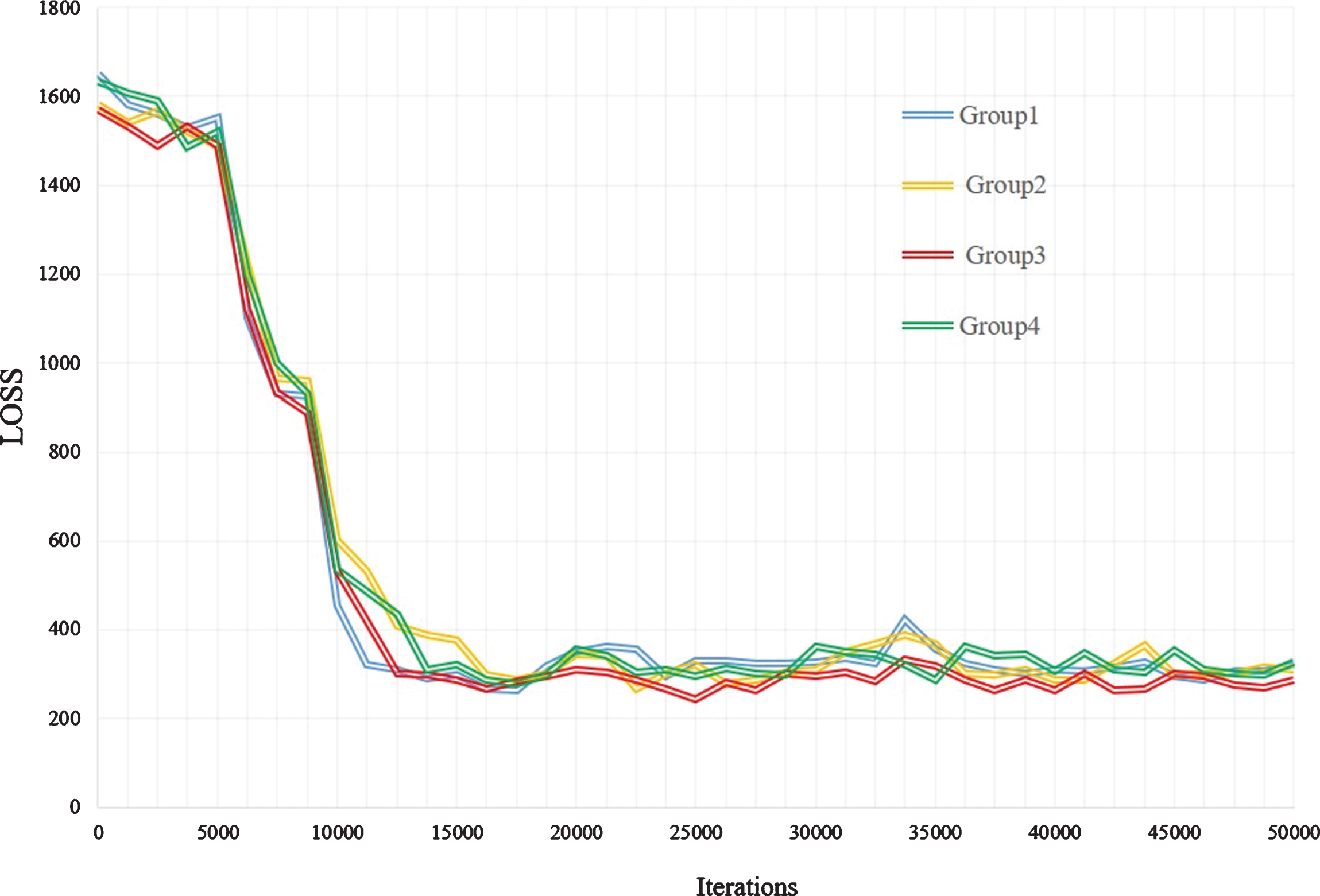
Training loss values based on different numbers of filters employed for network training.
The TV regularization term is essential for preserving the edge structure information in the images for diagnosis. The weight value λ3 is a critical trainable parameter that influences the preservation effect and is designed to control the balance between the image reconstruction and the enhancement. When λ3 is set too small, the effect of TV regularization will be insignificant, leading to minimal improvement in the image quality. By contrast, a very large λ3 will excessively suppress the image noise, and to some extent, interfere with the image reconstruction. Therefore, we resort to the cross validation [51] method to determine a suitable value by setting different λ3 values. For fairness, the parameter settings are set the same for each network except for λ3. We validate the performances of the networks by varying λ3 on 30 randomly selected LDCT images. The effect of λ3 is quantitatively assessed by plotting the average SSIM and RMSE of the denoising images in Fig. 11. As shown, the SSIM reaches the maximum value when λ3 = 0.5, indicating that the reconstructed images are structurally most similar to the NDCT images. In this case, the DRCNN model exhibits the best performance in preserving the structure in the LDCT images. The RMSE represents the accuracy and stability of the reconstruction to some extent. A lower RMSE indicates that the artifacts in the LDCT images are removed more completely. Given the image detail preservation and noise reduction of the LDCT images, we set λ3 to 0.5.
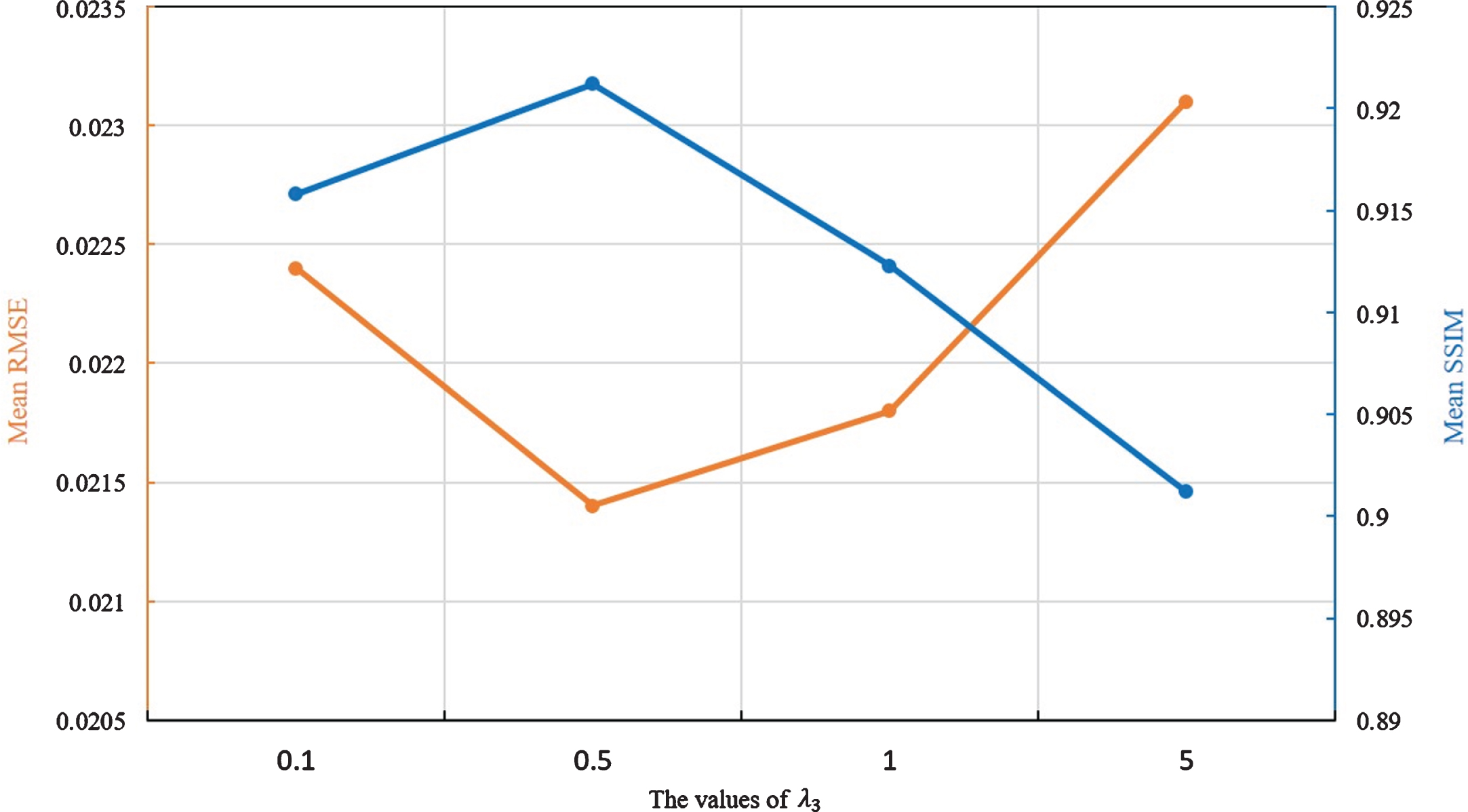
Influence of weight λ3 on the enhancement performance. The blue and orange lines represent the SSIM and RMSE curves, respectively.
In the field of modern medical CT imaging, the potential risks of radiation dose to patients have increased the requirements for LDCT. However, LDCT images inevitably contain severe noise, resulting in low-quality images and interfering with the clinical diagnosis. Although the deep neural network-based processing methods proposed in recent years represent a new solution for denoising LDCT images, most of the existing neural networks used for LDCT image reconstruction lead to loss of information or blurred details in the resulting images.
To achieve a higher LDCT image quality and extend the application scope of neural networks for LDCT noise reduction, in this study, we developed a new CT reconstruction network by incorporating sinogram-domain and image-domain sub-nets by integrating an analytical domain transform layer, which reduced computational time by training both sinogram-domain sub-net and image-domain sub-net simultaneously. The proposed DRCNN model contains three cascading units, each responsible for a specific task. Specifically, the forepart sinogram-domain process unit is used to learn the statistical information noise in sinogram image, which contributes to extract features from the sinogram and prevent the loss of projection information. And the domain transformation unit was accurately implemented via analytical back-projection algorithm, which was embedded in the proposed DRCNN model as a specific layer instead of being independent of the entire network to reduce the running time and preserve more necessary information. The final image-domain process unit can effectively capture spatial variations of noise forms of CT images and the global information of the whole CT image to reduce the residual errors in image while decrease the computational complexity. In the experiments conducted on simulation and real data, the visual effects showed that the DRCNN network can suppress the noise in the LDCT images and preserve more structural details. And the results of quantitative evaluations demonstrated that simultaneous training of sinogram-domain and image-domain subnets helped improve the PSNR by nearly 1 dB, compared with the state-of-the-art DP-ResNet method. Furthermore, it can be observed that DRCNN has significant statistical merits over other methods by comparing the P value in statistical analysis.
However, we recognize that the DRCNN network in the dual domain is somewhat empirical with no rigorous mathematical derivation as a support. Further investigations on reducing the calculation cost between the projections and back-projections are essential for constructing such an end-to-end network. Therefore, in further studies, we will focus on solving this problem by replacing the FBP transform layer with a convolution layer. Besides, in this work, we just considered the enhancement of the performance of a single image and ignore the internal information between CT slices. In the future, we hope to construct a new neural network to take full advantage of the similarity between CT slices while improving the reconstruction performance.
Regarding the training data employed in this study, the low-dose data were simulated from normal-dose data. However, the simulated data noise is different from the real case, and this mismatch may decrease the performance in practical applications. In the future, we will extend our DRCNN model to more clinical CT data and other medical CT image reconstruction tasks, such as the limited-angle CT image reconstruction [52], positron emission tomography (PET) [53], and single-photon emission-computed tomography (SPECT) [54] imaging.
Footnotes
Acknowledgments
This research was funded by National Science Foundation for Post-doctoral Scientists of China (Grant No. 2019M663996) and the National Natural Science Foundation of China (Grant No.61601518).