Observer-based control of polynomial fuzzy fractional-order systems

Abstract

In this study, the Lyapunov technique is used to analyze the observer-based control problem for polynomial fuzzy fractional order (PFFO) models. The case of polynomial matrices with unmeasurable states is considered to increase the applicability of the PFFO models in the design problem. In this regard, we offer two design procedures. First, the design conditions are presented in a one-step procedure. In this design, the non-convex conditions are transformed in a set of sum of squares (SOS) by introducing a new symbolic variable except the state vector $β$ and its estimated $\hat{β}$ . The obtained SOS conditions are presented involve three independent symbolic variables which increase both computing complexity and conservatism. To get around this shortcoming, a second design method is developed. By using the suggested method, SOS conditions requiring just two separate symbolic variables may be obtained. The architecture is shown in two stages; however, the observer and controller gains are computed in a single stage in order to further minimize conservatism. In order to demonstrate the utility of the suggested theoretical analysis, a simulated example is then provided.

Keywords

Fractional-order systems observer-based control sum of squares

Introduction

What does the fractional calculus term mean? It does not refer to fractional calculus. Neither does it refer to a portion of differential, integral, or calculus of variations. The term fractional calculus refers to the theory of integrals and derivatives of arbitrary order, which unifies and generalizes the concepts of integer-order differentiation and integration. In fact, fractional-order (FO) systems are dynamical systems that may be represented by fractional differential equations with non-integer derivatives (Kilbas et al., 2015; Podlubny, 1999). In this context, integral and differential equations that included FO derivative and integral operators emerge in the mathematical models of a variety of real-world processes and phenomena occurring in control theory, chemistry, blood flow problems, physics, signal and image processing, biophysics, electrodynamics, economics, aerodynamics, polymer rheology, and so on.

On the contrary, Takagi and Sugeno defined the fuzzy T-S model in 1985. Through using fuzzy sector nonlinearity notion, a nonlinear system may be precisely characterized as a collection of local linear subsystems linked by fuzzy membership functions in the form of a fuzzy T-S model. Numerous articles have examined the stability of fuzzy T-S systems and fuzzy control system (Chen et al., 2016; Elias et al., 2021 and references therein). Since not all states of process control are quantifiable in a real-world system, it is important to create an observer to approximate the states. Lin et al. (2005) suggested improvement on fuzzy observers through the fuzzy T-S model. Nonlinear integer-order systems have made extensive use of fuzzy control based on fuzzy T-S models. The fuzzy T-S approach is still effective for nonlinear FO systems; however, certain studies have been published on the analysis, control, and observer-based control of nonlinear FO systems Naifar et al. (2018). Indeed, the work in Fan and Wang (2022) has focused on analysis and control for T-S fuzzy FO systems by using fuzzy Lyapunov function. In addition, the investigation by Duan and Li (2018) has examined the observer-based control of this class of systems. Recently, the authors of Boulham et al. (2023) propose a fuzzy $L_{1}$ adaptive controller for FO chaotic models.

Polynomial fuzzy modeling is a generalization of the T-S fuzzy model (Chibani et al., 2018; Tanaka et al., 2009, 2012), which allows for more flexible and accurate modeling of complex nonlinear systems. In fact, to obtain standard T-S fuzzy model, all the nonlinearities must be decomposed. Consequently, if the number of nonlinearities is important, the number of local models will be also very important, and the observer-based control design problem could become very complex. Whereas, in polynomial fuzzy model, the matrices of local models are not constant, and thus, we do not need to decompose all the nonlinearities. So, the number of rules in polynomial fuzzy model is generally equal to or fewer than that in T-S fuzzy model.

To the best of our knowledge, there are no published works that discuss the observer-based control problem of FO polynomial fuzzy model when the parameters of the system matrices and control matrices are not measurable. In this context, to deal with FO polynomial fuzzy model, the sum of squares (SOS) approach is introduced. In fact, recent advances in positive polynomial theory, particularly the SOS theory, offer potentially viable methods for analyzing and synthesizing nonlinear polynomial systems. For example, a tracking controller is developed in Iben Ammar et al. (2021) for a DC–DC converter presented in polynomial form. The problem of observer-based control of polynomial fuzzy model is treated in Tanaka et al. (2012) and Liu and La (2015). All previous results are presented for ordinary derivative polynomial systems in which the obtained SOS conditions can be handled by a toolbox named SOSTOOLS (Papachristodoulou et al., 2021).

In this paper, the problem of observer-based control of FO polynomial fuzzy systems is introduced and investigated. The following points summarize the main contributions on the work:

The FO T-S fuzzy polynomial system problem has not yet been addressed in the literature. Accordingly, our current effort addresses and resolves this issue.

The system’s matrices depend on inaccessible states, which makes the problem more generic.

Notations: $Π_{n \times n}$ and $Δ_{SOS}$ correspond, respectively, to the set of $n \times n$ polynomial matrices and the set of SOS.

Problem formulation and preliminaries

Definition 1: (Kilbas et al., 2015; $ς$ -order Caputo derivative)

Given an interval $[0, c]$ of $R$ , the Caputo fractional derivative of an absolutely continuous $h$ of order $0 < ς < 1$ is defined by

_{0}^{C} D_{t}^{ς} h (t) = \frac{1}{Γ (1 - ς)} \int_{0}^{t} {(t - τ)}^{- ς} h' (τ) d τ, t \in [0, c]

(1)

Lemma 1: Alikhanov (2010) Let $ς \in (0, 1)$ and $P \in R^{n \times n}$ a constant, square, symmetric, and positive definite matrix. Then, the following relationship holds

\frac{1}{2}_{0}^{C} D_{t}^{ς} (x^{T} (t) P β (t)) \leq x^{T} (t) P_{0}^{C} D_{t}^{ς} β (t), t \geq 0

Definition 2: Kilbas et al. (2015) The Mittag-Leffler function is given by

E_{ς} (χ) = \sum_{k = 0}^{+ \infty} \frac{χ^{k}}{Γ (k ς + 1)}

Where, $ς > 0$ , $χ \in C$ .

Consider the system

\begin{matrix} _{0}^{C} D_{t}^{ς} β (t) = F (t, β), t \geq 0 \\ β (0) = β_{0} \end{matrix}

(2)

where, $F : R_{+} \times R^{n} \to R^{n}$ is a smooth enough to ensure the existence and uniqueness of global solutions for each initial condition $(0, β_{0})$ .

One presents the following definition related to the above nonlinear FO system.

Definition 3: Li et al. (2009) The FO system (2) is said to be Mittag-Leffler stable if there exists positive scalar $λ$ such that

∥ β (t) ∥ \leq {[m (β_{0}) E_{ς} (- λ t^{ς})]}^{b}, \forall t \geq 0

with $b > 0$ , $m (0) = 0$ , $m (β) \geq 0$ , and $m$ is locally Lipschitz.

Lemma 2: FO Lyapunov direct method

The equilibrium point $β = 0$ of FO system (2) is Mittag-Leffler stable if there exist a continuously differentiable function $V (β (t))$ , positive constants $α_{1}$ , $α_{2}$ , $α_{3}$ , $a$ , and $b$ such that

α_{1} ∥ β (t) ∥^{a} \leq V (β (t)) \leq α_{2} ∥ β (t) ∥^{ab}

(3)

_{0}^{C} D_{t}^{ς} β (t) \leq - α_{3} ∥ β (t) ∥^{ab}

(4)

Lemma 3: Tanaka et al. (2012) Let $G (β) \in Π_{n \times n}$ . The following inequality

G (β) < 0

(5)

holds if the following SOS condition

- η^{T} (G (β) - ϵ (β)) η \in Δ_{SOS}

(6)

is satisfied

where $η \in R^{n}$ is a vector independent of $β$ , and $ϵ (β)$ is predefined scalar polynomial.

Consider the FO polynomial fuzzy model as follows:

Plant rule $i (i = 1, 2, \dots, w)$ : If $κ_{1} (t)$ is $μ_{i 1}$ and $κ_{p} (t)$ is $μ_{ip}$ then

{\begin{matrix} _{0}^{C} D_{t}^{ς} β (t) = A_{i} (β (t)) β (t) + B_{i} (β (t)) u (t) \\ y (t) = C β (t) \end{matrix}

(7)

where $κ_{j} (t)$ , $w$ , and $μ_{ij} (i = 1, \dots, r, j = 1, \dots, p)$ are, respectively, the premise variables, the total numbers of rules, and the fuzzy sets. $β (t) \in R^{n_{β}}$ , $u (t) \in R^{n_{u}}$ , and $y (t) \in R^{n_{y}}$ represent, respectively, the state of system, the control input, and the measurement output vector. $A_{i} (β (t)) \in Π_{n_{β} \times n_{β}}$ and $B_{i} (β (t)) \in Π_{n_{β} \times n_{u}}$ , and $C$ is known constant matrix with compatible size such as $rank (C) = n_{y}$ . A singular value decomposition of $C$ is a factorization

C = U_{1} [\begin{matrix} D & 0 \end{matrix}] U_{2}^{T}

(8)

where $U_{1}$ is an $n_{y} \times n_{y}$ orthogonal matrix, $U_{2}$ is an $n_{β} \times n_{β}$ orthogonal matrix, $D = diag (c_{1}, c_{2}, \dots, c_{n_{y}})$ and $c_{i} (i = 1, \dots, n_{y})$ are nonzero singular values of $C$ .

Remark 1: The following form of model

Plant Rule $i (i = 1, 2, \dots, w)$ : If $κ_{1} (t)$ is $μ_{i 1}$ and $κ_{p} (t)$ is $μ_{ip}$ THEN

{\begin{matrix} _{0}^{C} D_{t}^{ς} β (t) = A_{i} (β (t)) \bar{β} (β (t)) + B_{i} (β (t)) u (t) \\ y (t) = C \bar{β} (β (t)) \end{matrix}

is more general than the form (7), where $\bar{β} (β (t))$ is a monomial vector in $β (t)$ .

In this paper, we adopt the simpler representation to focus our attention on the design procedure.

The FO polynomial fuzzy model (7) can be inferred as follows

{\begin{matrix} _{0}^{C} D_{t}^{ς} β (t) = \sum_{i = 1}^{w} δ_{i} (κ (t)) (A_{i} (β (t)) β (t) + B_{i} (β (t)) u (t)) \\ y (t) = C β (t) \end{matrix}

(9)

where

δ_{i} (κ (t)) \geq 0, \sum_{i = 1}^{w} δ_{i} (κ (t)) = 1

(10)

For brevity, we will drop the notation with respect to time $t$ , and we will use $δ_{i}$ to denote $δ_{i} (κ (t))$ .

To estimate the states of system (9), we consider the following FO polynomial fuzzy observer

{\begin{matrix} _{0}^{C} D_{t}^{ς} \hat{β} = \sum_{i = 1}^{w} δ_{i} (A_{i} (\hat{β}) \hat{β} + B_{i} (\hat{β}) u + L_{i} (\hat{β}) y_{e}) \\ \hat{y} = C \hat{β} \\ y_{e} = y - \hat{y} \end{matrix}

(11)

where $\hat{β}$ , $\hat{y}$ , and $L_{i} (\hat{β})$ are, respectively, the estimated state, the estimated output vector, and the polynomial observer gains to be designed.

To stabilize FO polynomial system (9), we consider the following polynomial fuzzy controller

u = - \sum_{i = 1}^{w} δ_{i} K_{i} (\hat{β}) \hat{β}

We define $β_{e} = β - \hat{β}$ . The augmented system can be described as

_{0}^{C} D_{t}^{ς} \tilde{β} = \sum_{i = 1}^{w} \sum_{j = 1}^{w} δ_{i} δ_{j} {\tilde{A}}_{ij} (\tilde{β}) \tilde{β}

(12)

where

\tilde{β} = [\begin{matrix} \hat{β} \\ β_{e} \end{matrix}], {\tilde{A}}_{ij} (\tilde{β}) = [\begin{matrix} A_{i} (\hat{β}) - B_{i} (\hat{β}) K_{j} (\hat{β}) & L_{i} (\hat{β}) C \\ {\tilde{A}}_{ij}^{12} (\tilde{β}) & A_{i} (β) - L_{i} (\hat{β}) C \end{matrix}]

in which

{\tilde{A}}_{ij}^{12} (\tilde{β}) = (A_{i} (β) - A_{i} (\hat{β})) - (B_{i} (β) - B_{i} (\hat{β})) K_{j} (\hat{β})

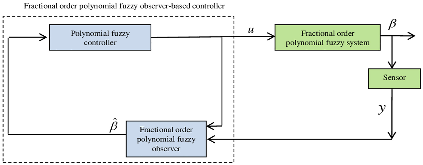
The control structure diagram is given in Figure 1.

Main results

Theorem 1: The closed-loop system (12) is Mittag-Leffler stable if there exist positive symmetric definite matrices $X_{1} \in R^{n_{β} \times n_{β}}$ , $X_{2}^{11} \in R^{n_{y} \times n_{y}}$ , $X_{2}^{22} \in R^{(n_{β} - n_{y}) \times (n_{β} - n_{y})}$ , $X_{2}^{21} \in R^{(n_{β} - n_{y}) \times (n_{y})}$ $Q$ , polynomial matrices ${\tilde{L}}_{i} (\hat{β})$ , ${\tilde{K}}_{i} (\hat{β})$ such that the following SOS-based conditions are satisfied

η_{1}^{T} (X_{1} - ϵ_{1} I) η_{1} \in Δ_{SOS}

(13)

η_{1}^{T} (X_{2} - ϵ_{2} I) η_{1} \in Δ_{SOS}

(14)

η_{1}^{T} (Q - ϵ_{3} I) η_{1} \in Δ_{SOS}

(15)

- η_{2}^{T} (Ω_{ij} (\tilde{β}) + Ω_{ji} (\tilde{β}) + Q + ϵ_{4 ij} (\tilde{β}) I) η_{2} \in Δ_{SOS}, i \leq j

(16)

where $η_{1}$ and $η_{2}$ denote vectors that are independent of $\tilde{β}$ ; $ϵ_{1} > 0$ , $ϵ_{2} > 0$ $ϵ_{3} > 0$ , and $ϵ_{4 ij} > 0$ are predefined scalar polynomials

X_{2} = U_{2} [\begin{matrix} X_{2}^{11} & 0 \\ 0 & X_{2}^{22} \end{matrix}] U_{2}^{T}

Ω_{ij} (\tilde{β}) = [\begin{matrix} Ω_{ij}^{11} (\hat{β}) & Ω_{ij}^{12} (\tilde{β}) \\ * & Ω_{ij}^{22} (\tilde{β}) \end{matrix}]

in which

\begin{matrix} Ω_{ij}^{11} (\hat{β}) = Sym (A_{i} (\hat{β}) X_{1} - B_{i} (\hat{β}) {\tilde{K}}_{j} (\hat{β})) \\ Ω_{ij}^{12} (\tilde{β}) = {\tilde{L}}_{i} (\hat{β}) C + X_{1} (A_{i} (β) - A_{i} (\hat{β}))^{T} - {\tilde{K}}_{j}^{T} (\hat{β}) (B_{i} (β) - B_{i} (\hat{β}))^{T} \\ Ω_{ij}^{22} (\tilde{β}) = Sym (A_{i} (β) X_{2} - {\tilde{L}}_{i} (\hat{β}) C) \end{matrix}

In this case, the gains of the polynomial fuzzy observer-based controller are given by $L_{i} (\hat{β}) = {\tilde{L}}_{i} (\hat{β}) U_{1} D (X_{2}^{11})^{- 1} D^{- 1} U_{1}^{T}$ and $K_{i} (\hat{β}) = {\tilde{K}}_{i} (\hat{β}) X_{1}^{- 1}$

Proof: We consider the following Lyapunov function

V (\tilde{β}) = {\tilde{β}}^{T} P \tilde{β}

(17)

where

P = [\begin{matrix} P_{1} & 0 \\ 0 & P_{2} \end{matrix}]

in which $X_{1} = P_{1}^{- 1}$ , $X_{2} = P_{2}^{- 1}$ .

The conditions (13) and (14) imply that $V (\tilde{β})$ is positive definite $\forall \tilde{β}$ .

$P_{2}$ is written in the following form

P_{2} = U_{2} [\begin{matrix} P_{2}^{11} & 0 \\ 0 & P_{2}^{22} \end{matrix}] U_{2}^{T}

It is clear that

λ_{\min} (P) ∥ \tilde{β} ∥^{2} \leq V (\tilde{β}) \leq λ_{\max} (P) ∥ \tilde{β} ∥^{2}

From Lemma 1

_{0}^{C} D_{t}^{ς} V (\tilde{β}) \leq 2 {\tilde{β}}^{T} P_{0}^{C} D_{t}^{ς} \tilde{β}

(18)

Combining equations (18) and (12) yields

\begin{array}{l} _{0}^{C} D_{t}^{ς} V (\tilde{β}) \leq \sum_{i = 1}^{w} \sum_{j = 1}^{w} δ_{i} δ_{j} {\tilde{β}}^{T} Φ_{i j} (x, \overset{⌣}{x}) \tilde{β} \\ = \sum_{i = 1}^{w} \sum_{i \leq j}^{w} δ_{i} δ_{j} {\tilde{β}}^{T} (Φ_{i j} (\tilde{β}) + Φ_{j i} (\tilde{β})) \tilde{β} \end{array}

where

Φ_{ij} (\tilde{β}) = [\begin{matrix} Φ_{ij}^{11} (\hat{β}) & Φ_{ij}^{12} (\tilde{β}) \\ * & Φ_{ij}^{22} (\tilde{β}) \end{matrix}]

in which

Φ_{ij}^{11} (\hat{β}) = Sym (P_{1} (A_{i} (\hat{β}) - B_{i} (\hat{β}) K_{j} (\hat{β})))

Φ_{ij}^{12} (\tilde{β}) = P_{1} L_{i} (\hat{β}) C + ({\tilde{A}}_{ij}^{12} (\tilde{β}))^{T} P_{2}

Φ_{ij}^{22} (\tilde{β}) = P_{2} (A_{i} (β) - L_{i} (\hat{β}) C)

Let $X = [\begin{matrix} X_{1} & 0 \\ 0 & X_{2} \end{matrix}]$ , then equation (19) can be written as

_{0}^{C} D_{t}^{ς} V (\tilde{β}) \leq \sum_{i = 1}^{w} \sum_{i \leq j}^{w} δ_{i} δ_{j} ζ^{T} (Ξ_{ij} (\tilde{β}) + Ξ_{ji} (\tilde{β})) ζ

(19)

where

ζ = X^{- 1} \tilde{β}, Ξ_{ij} (\tilde{β}) = [\begin{matrix} Ω_{ij}^{11} (\hat{β}) & Ξ_{ij}^{12} (\tilde{β}) \\ * & Ξ_{ij}^{22} (\tilde{β}) \end{matrix}]

in which

\begin{matrix} Ξ_{ij}^{12} (\tilde{β}) = L_{i} (\hat{β}) C X_{2} + X_{1} ({\tilde{A}}_{ij}^{12} (\tilde{β}))^{T} \\ Ξ_{ij}^{22} (\tilde{β}) = Sym (A_{i} (β) X_{2} - L_{i} (\hat{β}) C X_{2}) \end{matrix}

From equation (8), we get

\begin{matrix} L_{i} (\hat{β}) C X_{2} = L_{i} (\hat{β}) U_{1} [\begin{matrix} D & 0 \end{matrix}] U_{2}^{T} U_{2} [\begin{matrix} X_{2}^{11} & 0 \\ 0 & X_{2}^{22} \end{matrix}] U_{2}^{T} \\ = L_{i} (\hat{β}) U_{1} [D X_{2}^{11} 0] U_{2}^{T} \\ = L_{i} (\hat{β}) U_{1} D X_{2}^{11} D^{- 1} U_{1}^{T} U_{1} [\begin{matrix} D & 0 \end{matrix}] U_{2}^{T} \end{matrix}

Define ${\tilde{L}}_{i} (\hat{β}) = L_{i} (\hat{β}) U_{1} D X_{2}^{11} D^{- 1} U_{1}^{T}$ , we obtain

L_{i} (\hat{β}) C X_{2} = {\tilde{L}}_{i} (\hat{β}) C

(20)

Considering the previous equality, equation (19) can written as

_{0}^{C} D_{t}^{ς} V (\tilde{β}) \leq \sum_{i = 1}^{w} \sum_{i \leq j}^{w} δ_{i} δ_{j} ζ^{T} (Ω_{ij} (\tilde{β}) + Ω_{ji} (\tilde{β})) ζ

(21)

Since the SOS conditions (16) imply that $Ω_{ij} (\tilde{β}) + Ω_{ji} (\tilde{β}) < - Q$ and by considering $δ_{i} (κ (t)) \geq 0$ , $\sum_{i = 1}^{w} δ_{i} (κ (t)) = 1$ , we get

_{0}^{C} D_{t}^{ς} V (\tilde{β}) \leq - λ_{\min} (Q) ∥ X^{- 1} ∥^{2} ∥ \tilde{β} ∥^{2}

(22)

It is clear from equation (15) that $λ_{\min} (Q) > 0$ . Then, according to Lemma 2, the closed-loop FO polynomial fuzzy system (12) is Mittag-Leffler stable. The proof is completed.

Remark 2: It is well known that the stability and stabilization conditions of the polynomial fuzzy systems are commonly derived based on polynomial Lyapunov functions. However, we notice, for observer-based control problem, the use of a polynomial Lyapunov function is not evident. In fact, the states $β$ are not measurable, and we cannot use the polynomial Lyapunov matrix $P (β)$ .

Remark 3: The main disadvantage of this result is the introduction of symbolic vector $η_{2}$ independent of $β$ and $\hat{β}$ which can significantly increase the computational demand.

To overcome this drawback, 2-step procedure is proposed in the following theorem:

Theorem 2: The closed-loop system (12) is Mittag-Leffer stable if there exists a feasible solution to the following 2-step procedure:

First step: There exist positive symmetric definite matrices $X_{1}$ , $X_{2}$ , $Q$ , polynomial matrices ${\tilde{L}}_{i} (β)$ , ${\tilde{K}}_{i} (β)$ such that equations (13)–(15) and the following SOS-based conditions are satisfied

- η_{2}^{T} (Ψ_{ij} (β) + Ψ_{ji} (β) + Q + ϵ_{4 ij} (β) I) η_{2} \in Δ_{SOS}, i \leq j

(23)

where

Ψ_{ij} (β) = [\begin{matrix} Ψ_{ij}^{11} (β) & {\tilde{L}}_{i} (β) C \\ * & Ψ_{ij}^{22} (β) \end{matrix}]

in which

\begin{matrix} Ψ_{ij}^{11} (β) = Sym (A_{i} (β) X_{1} - B_{i} (β) {\tilde{K}}_{j} (β)) \\ Ψ_{ij}^{12} (β) = {\tilde{L}}_{i} (β) C \\ Ψ_{ij}^{22} (β) = Sym (A_{i} (β) X_{2} - {\tilde{L}}_{i} (β) C) \end{matrix}

Second step: $X_{1}$ and $X_{2}$ are known matrices obtained in step 1.

If there exist positive symmetric definite matrix $Q$ , polynomial matrices ${\tilde{L}}_{i} (\hat{β})$ and ${\tilde{K}}_{i} (\hat{β})$ such that equation (15) and the following SOS-based conditions are satisfied

- ζ^{T} (Ω_{ij} (\tilde{β}) + Ω_{ji} (\tilde{β}) + Q + ϵ_{4 ij} (\tilde{β}) I) ζ \in Δ_{SOS}, i \leq j

(24)

In this case, the gains of the polynomial fuzzy observer-based controller are given as in Theorem 1.

Proof: The first step is directly obtained from Theorem 1 and by assuming that all the states are measurable (e.g. $β = \hat{β}$ and $X_{1} (A_{i} (β) - A_{i} (\hat{β}))^{T} - {\tilde{K}}_{j}^{T} (\hat{β}) (B_{i} (β) - B_{i} (\hat{β}))^{T} = 0$ ).

Since $X_{1}$ and $X_{2}$ are known matrices, then $ζ^{T} (Ω_{i j} (\tilde{β}) + Ω_{j i} (\tilde{β})) ζ < 0$ is linear polynomial matrix inequality and can be guaranteed by SOS condition (24).

Now, we suppose that the consequent parts in the FO polynomial fuzzy model depend only on measurable variables, that is, $A_{i} (β) = A_{i} (y), B_{i} (β) = B_{i} (y)$ . In this case, The augmented system can be described as

_{0}^{C} D_{t}^{ς} \tilde{β} = \sum_{i = 1}^{w} \sum_{j = 1}^{w} δ_{i} δ_{j} {\tilde{A}}_{ij} (y) \tilde{β}

(25)

where

{\tilde{A}}_{ij} (y) = [\begin{matrix} A_{i} (y) - B_{i} (y) K_{j} (y) & L_{i} (y) C \\ 0 & A_{i} (y) - L_{i} (y) C \end{matrix}]

Corollary 1: The closed-loop system (25) is Mittag-Leffer stable if there exist positive symmetric definite matrices $X_{1}$ , $X_{2}$ , polynomial matrices ${\tilde{L}}_{i} (y)$ , ${\tilde{K}}_{i} (y)$ such that equations (13)–(15) and the following SOS-based conditions are satisfied

- η_{2}^{T} (Λ_{ij} (y) + Λ_{ji} (y) + ϵ_{4 ij} (y) I) η_{2} \in Δ_{SOS}, i \leq j

(26)

where

Λ_{ij} (y) = [\begin{matrix} Sym (A_{i} (y) X_{1} - B_{i} (y) {\tilde{K}}_{j} (y)) & - {\tilde{L}}_{i} (y) C \\ * & Sym (A_{i} (y) X_{2} - {\tilde{L}}_{i} (y) C) \end{matrix}]

In this case, the gains of the polynomial fuzzy observer-based controller are given as in Theorem 1.

Discussion and main contributions

The following condition

- {\tilde{β}}^{T} (Ω_{ij} (\tilde{β}) + Ω_{ji} (\tilde{β}) + ϵ_{3 ij} (\tilde{β}) I) \tilde{β} \in Δ_{SOS}

does not always imply that $Ω_{ij} (\tilde{β}) + Ω_{ji} (\tilde{β}) < 0$ . $Ω_{ij} (\tilde{β})$ must be constant matrices for this to be a necessary and sufficient condition. Except in this instance, there is no conservatism. For other cases, as in Theorem 1, we have to introduce a vector $η_{2}$ independent of $\tilde{β}$

- η_{2}^{T} (Ω_{ij} (\tilde{β}) + Ω_{ji} (\tilde{β}) + ϵ_{3 ij} (\tilde{β}) I) η_{2} \in Δ_{SOS}

The presence of a vector $η_{2}$ and the term $(A_{i} (β) - A_{i} (\hat{β})) X_{1} - (B_{i} (β) - B_{i} (\hat{β})) {\tilde{K}}_{j} (\hat{β})$ at the same time, in the previous SOS conditions, is a main source of conservatism and computational complexity. The Theorem 2 provides a technique to circumvent this primary issue.

Theorem 2 can be applied when the order is equal to one, that is, the model and the observer-based controller are as follows, respectively

{\begin{matrix} \overset{\cdot}{x} = \sum_{i = 1}^{w} δ_{i} (A_{i} (β) β (t) + B_{i} (β) u) \\ y = C x, \end{matrix}

(27)

and

{\begin{matrix} \overset{\cdot}{\hat{β}} = \sum_{i = 1}^{w} δ_{i} (A_{i} (\hat{β}) \hat{β} + B_{i} (\hat{β}) u + L_{i} (\hat{β}) y_{e}) \\ \hat{y} = C \hat{β} \\ y_{e} = y - \hat{y} \\ u = - \sum_{i = 1}^{w} δ_{i} K_{i} (\hat{β}) \hat{β} \end{matrix}

(28)

In this case, the main contributions compared with existing results can be summarized as follows:

Compared with Tanaka et al. (2012), in the first step, the authors design polynomial controller by determining a constant matrix $X_{1}$ and polynomial matrices $K_{i} (β)$ in the first phase, then they replace $K_{i} (β)$ with $K_{i} (\hat{β})$ and determine the matrices $X_{2}$ and $L_{j} (\hat{β})$ . In our example, we begin by identifying the constant matrices $X_{1}$ and $X_{2}$ , then the polynomial matrices $K_{i} (\hat{β})$ and $L_{i} (\hat{β})$ , which allows us to provide greater freedom in the second phase.

Compared with Liu and La (2015), the vector $η_{2}$ and the term $(A_{i} (β) - A_{i} (\hat{β})) X_{1} - (B_{i} (β) - B_{i} (\hat{β})) {\tilde{K}}_{j} (\hat{β})$ are presented at the same time, in the SOS conditions, which increase not only the complexity of the SOS but also the conservatism. A numerical example is taken to confirm the statement in this remark.

Illustrative example

The following nonlinear system is considered to verify the proposed observer-based controller designed method

{\begin{matrix} {\overset{\cdot}{β}}_{1} = \sin (β_{1}) - 0.3 β_{2}^{2} + (β_{1}^{2} + 1) u \\ {\overset{\cdot}{β}}_{2} = - 1.5 β_{1} - (2 + β_{2}^{2}) β_{2} \\ y = β_{1} \end{matrix}

(29)

which can be represented by the following model

{\begin{matrix} \overset{\cdot}{β} = \sum_{i = 1}^{2} δ_{i} {A_{i} (β) β + B_{i} (β) u} \\ y = C β \end{matrix}

(30)

where $β = {[\begin{matrix} β_{1} & β_{2} \end{matrix}]}^{T}$

\begin{matrix} A_{1} (β) = [\begin{matrix} 1 & - 0.3 β_{2} \\ - 1.5 & - 2 - β_{2}^{2} \end{matrix}], A_{2} (β) = [\begin{matrix} - 0.2172 & - 0.3 β_{2} \\ - 1.5 & - 2 - β_{2}^{2} \end{matrix}] \\ B_{1} (β) = B_{2} (β) = [\begin{matrix} β_{1}^{2} + 1 \\ 0 \end{matrix}], C = [\begin{matrix} 1 & 0 \end{matrix}] \\ δ_{1} = \frac{\sin (y) + 0.2172 y}{1.2172 y}; δ_{2} = \frac{y - \sin (y)}{1.2172 y} \end{matrix}

Tanaka et al. (2012) and Liu and La (2015) cannot produce set of feasible solutions. Now, by applying Theorem 2, we obtain the following set of feasible solutions

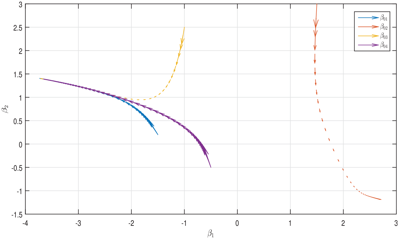
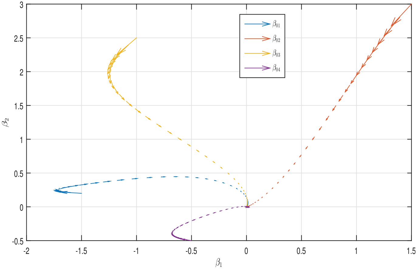
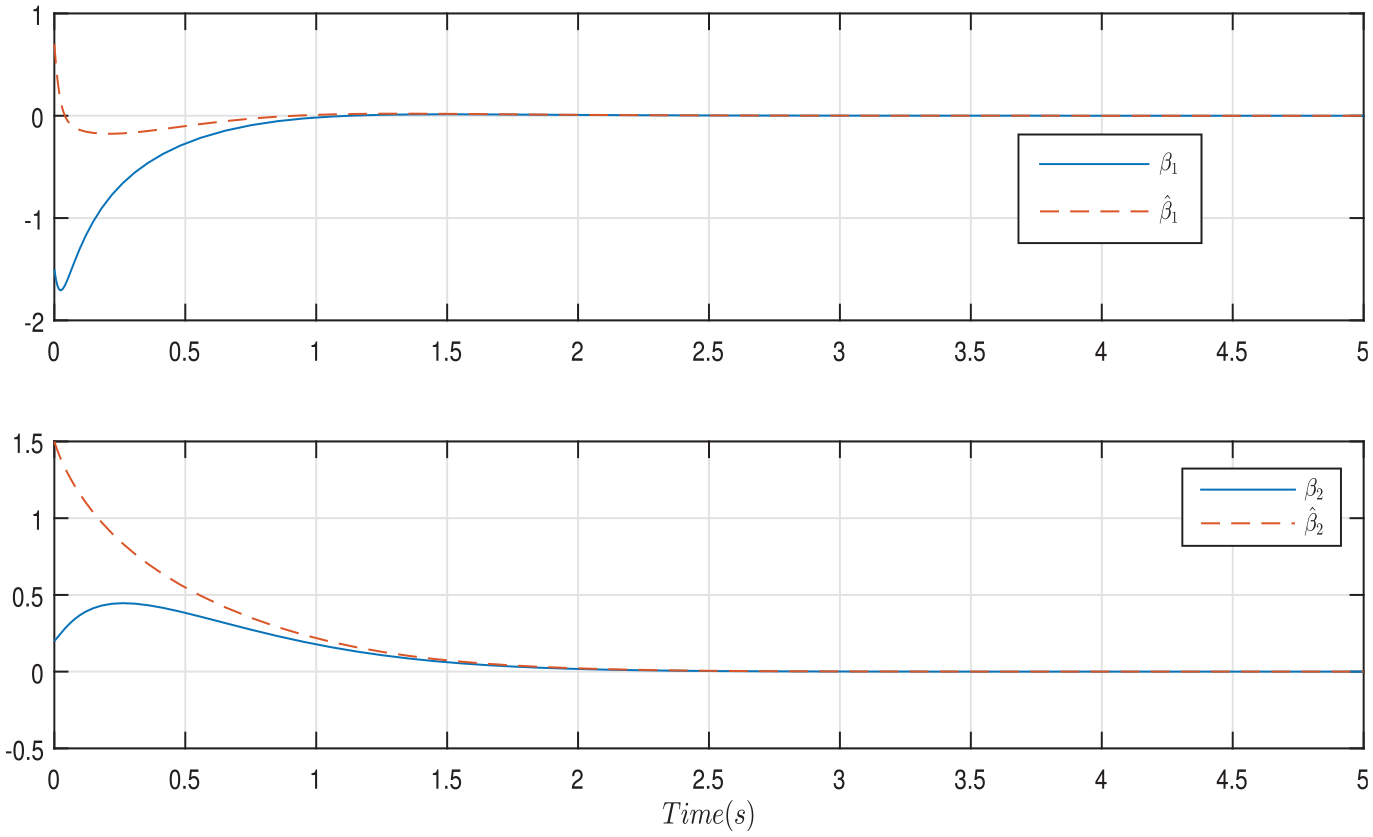
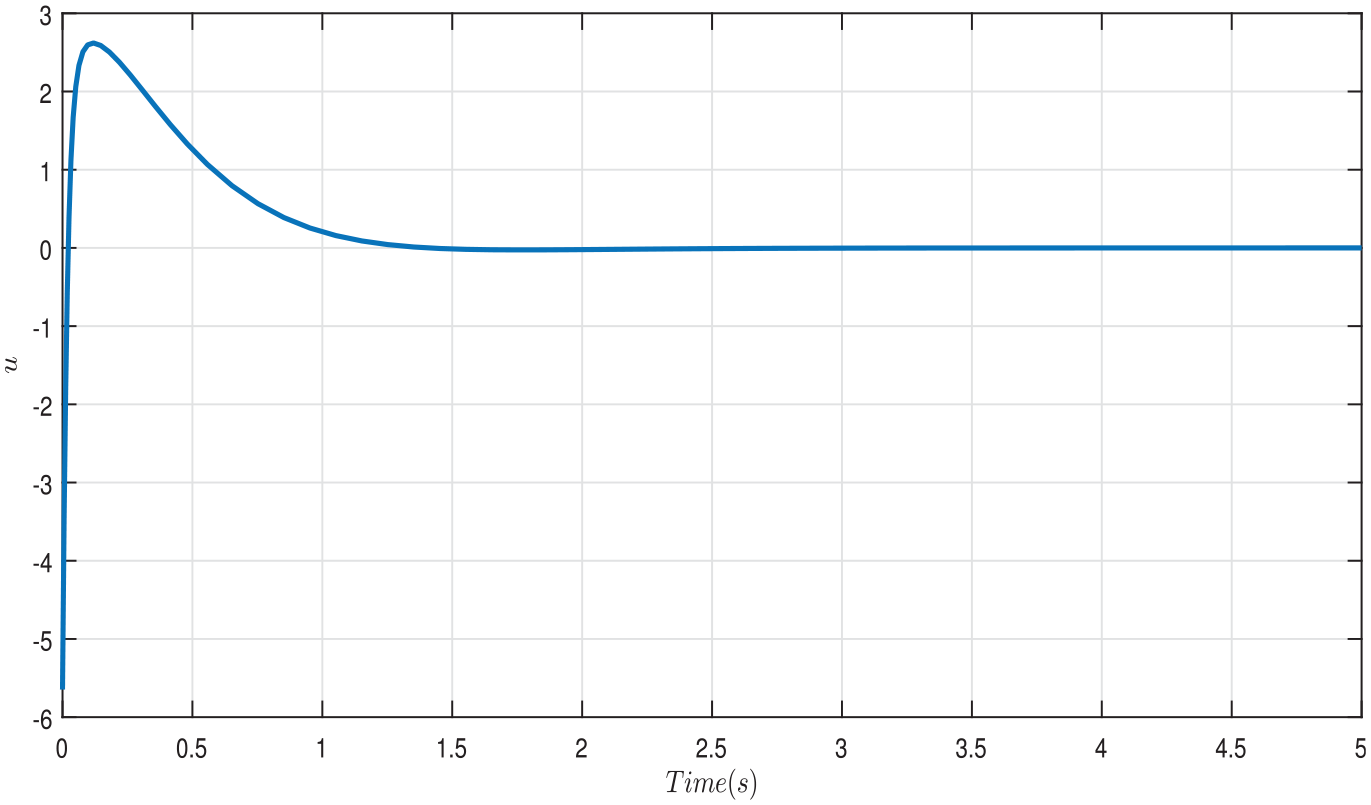
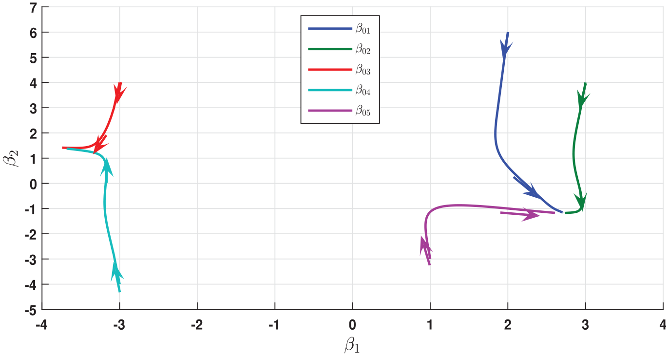
\begin{matrix} K_{1} (\hat{β}) = [\begin{matrix} 2.3592 {\hat{β}}_{2}^{2} + 0.0225 {\hat{β}}_{2} + 5.249 & - 0.0011 {\hat{β}}_{2}^{2} - 0.141 {\hat{β}}_{2} - 1.122 \end{matrix}] \\ K_{2} (\hat{β}) = [\begin{matrix} 3.194 {\hat{β}}_{2}^{2} + 0.013 {\hat{β}}_{2} + 3.943 & - 0.0015 {\hat{β}}_{2}^{2} - 0.001 {\hat{β}}_{2} - 1.013 \end{matrix}] \\ L_{1} (\hat{β}) = [\begin{matrix} 1.772 {\hat{β}}_{2}^{2} + 0.016 {\hat{β}}_{2} + 4.254 \\ 0.016 {\hat{β}}_{2}^{2} - 0.068 {\hat{β}}_{2} - 0.894 \end{matrix}] \\ L_{2} (\hat{β}) = [\begin{matrix} 1.700 {\hat{β}}_{2}^{2} + 0.0054 {\hat{β}}_{2} + 2.997 \\ 0.104 \times 10^{- 3} {\hat{β}}_{2}^{2} + 0.074 {\hat{β}}_{2} - 0.902 \end{matrix}] \end{matrix}

Simulations results are presented in Figures 2 –5. Figure 2 shows the $β_{1} - β_{2}$ phase plane for polynomial fuzzy (PF) model (30) with $u = 0$ for different initial conditions $β_{01} = [\begin{matrix} - 1.5 & 0.2 \end{matrix}],$ $β_{02} = [\begin{matrix} 1.5 & 3 \end{matrix}], β_{03} = [\begin{matrix} - 1 & 2.5 \end{matrix}], β_{04} = [\begin{matrix} - 0.5 & - 0.5 \end{matrix}]$ . It is clear that unforced open-loop system (30) is not stable. Figure 3 depicts the $β_{1} - β_{2}$ phase plane for PF model (30) with the designed stabilizing controller for the same initial conditions. The system states $β$ and their estimation, for the initial conditions $β_{0} = [\begin{matrix} - 1.5 & 0.2 \end{matrix}], {\hat{β}}_{0} = [\begin{matrix} 0.7 & 1.5 \end{matrix}]$ , are illustrated in Figure 4. The control input is shown in Figure 5.

Now, we suppose that the order is not equal to one $(ς = 0.9)$

{\begin{matrix} \frac{d^{ς} β_{1}}{dt} = \sin (β_{1}) - 0.3 β_{2}^{2} + (β_{1}^{2} + 1) u \\ \frac{d^{ς} β_{2}}{dt} = - 1.5 β_{1} - (2 + β_{2}^{2}) β_{2} \\ y = β_{2} \end{matrix}

(31)

Suppose that $β_{2} \in [\begin{matrix} {\underline{β}}_{2}, & {\bar{β}}_{2} \end{matrix}]$ , $β_{2}^{2} \in [\begin{matrix} {\underline{β}}_{22}, & {\bar{β}}_{22} \end{matrix}]$ , and $β_{1}^{2} \in [\begin{matrix} {\underline{β}}_{12}, & {\bar{β}}_{12} \end{matrix}]$ . In this case, the FO nonlinear system (31) is described by the following FO T-S fuzzy model with unmeasurable premise variables

{\begin{matrix} _{0}^{C} D_{t}^{ς} β = \sum_{i = 1}^{16} θ_{i} {A_{i} β + B_{i} u} \\ y = C β \end{matrix}

(32)

where

\begin{matrix} A_{1} = A_{9} = [\begin{matrix} 1 & - 0.3 {\bar{β}}_{2} \\ - 1.5 & - 2 - {\bar{β}}_{22} \end{matrix}], A_{2} = A_{10} = [\begin{matrix} 1 & - 0.3 {\bar{β}}_{2} \\ - 1.5 & - 2 - {\underline{β}}_{22} \end{matrix}] \end{matrix}

\begin{matrix} A_{3} = A_{11} = [\begin{matrix} 1 & - 0.3 {\underline{β}}_{2} \\ - 1.5 & - 2 - {\underline{β}}_{22} \end{matrix}], A_{4} = A_{12} = [\begin{matrix} 1 & - 0.3 {\underline{β}}_{2} \\ - 1.5 & - 2 - {\bar{β}}_{22} \end{matrix}] \end{matrix}

\begin{matrix} A_{5} = A_{13} = [\begin{matrix} - 0.2172 & - 0.3 {\bar{β}}_{2} \\ - 1.5 & - 2 - {\bar{β}}_{22} \end{matrix}], \\ A_{6} = A_{14} = [\begin{matrix} - 0.2172 & - 0.3 {\bar{β}}_{2} \\ - 1.5 & - 2 - {\underline{β}}_{22} \end{matrix}] \end{matrix}

\begin{matrix} A_{7} = A_{15} = [\begin{matrix} - 0.2172 & - 0.3 {\underline{β}}_{2} \\ - 1.5 & - 2 - {\underline{β}}_{22} \end{matrix}], \\ A_{8} = A_{16} = [\begin{matrix} - 0.2172 & - 0.3 {\underline{β}}_{2} \\ - 1.5 & - 2 - {\bar{β}}_{22} \end{matrix}] \end{matrix}

\begin{matrix} θ_{1} = δ_{1} \times δ_{3} \times δ_{5} \times δ_{7}, θ_{2} = δ_{1} \times δ_{3} \times δ_{6} \times δ_{7}, \\ θ_{3} = δ_{1} \times δ_{4} \times δ_{6} \times δ_{7}, θ_{1} = δ_{1} \times δ_{4} \times δ_{5} \times δ_{7} \end{matrix}

\begin{matrix} θ_{5} = δ_{2} \times δ_{3} \times δ_{5} \times δ_{7}, θ_{6} = δ_{2} \times δ_{3} \times δ_{6} \times δ_{7}, \\ θ_{7} = δ_{2} \times δ_{4} \times δ_{6} \times δ_{7}, θ_{8} = δ_{2} \times δ_{4} \times δ_{5} \times δ_{7} \end{matrix}

\begin{matrix} θ_{9} = δ_{1} \times δ_{3} \times δ_{5} \times δ_{8}, θ_{10} = δ_{1} \times δ_{3} \times δ_{6} \times δ_{8}, \\ θ_{11} = δ_{1} \times δ_{4} \times δ_{6} \times δ_{8}, θ_{12} = δ_{1} \times δ_{4} \times δ_{5} \times δ_{8} \end{matrix}

\begin{matrix} θ_{13} = δ_{2} \times δ_{3} \times δ_{5} \times δ_{8}, θ_{14} = δ_{2} \times δ_{3} \times δ_{6} \times δ_{8}, \\ θ_{15} = δ_{2} \times δ_{4} \times δ_{6} \times δ_{8}, θ_{16} = δ_{2} \times δ_{4} \times δ_{5} \times δ_{8} \end{matrix}

\begin{matrix} B_{k_{1}} = [\begin{matrix} {\bar{β}}_{12} + 1 \\ 0 \end{matrix}], k_{1} = 1, \dots, 8; B_{k_{2}} = [\begin{matrix} {\underline{β}}_{12} + 1 \\ 0 \end{matrix}], \\ k_{2} = 9, \dots, 16 \end{matrix}

in which

\begin{matrix} δ_{1} = \frac{\sin (β_{1}) + 0.2172 β_{1}}{1.2172 β_{1}}, δ_{2} = \frac{β_{1} - \sin (β_{1})}{1.2172 β_{1}}, \\ δ_{3} = \frac{β_{2} - {\underline{β}}_{2}}{{\bar{β}}_{2} - {\underline{β}}_{2}}, δ_{4} = \frac{{\bar{β}}_{2} - β_{2}}{{\bar{β}}_{2} - {\underline{β}}_{2}} \\ δ_{5} = \frac{β_{2}^{2} - {\underline{β}}_{22}}{{\bar{β}}_{22} - {\underline{β}}_{22}}, δ_{6} = \frac{{\bar{β}}_{22} - β_{2}^{2}}{{\bar{β}}_{22} - {\underline{β}}_{22}}, δ_{7} = \frac{β_{1}^{2} - {\underline{β}}_{12}}{{\bar{β}}_{12} - {\underline{β}}_{12}}, \\ δ_{8} = \frac{{\bar{β}}_{12} - β_{1}^{2}}{{\bar{β}}_{12} - {\underline{β}}_{12}} \end{matrix}

The system (31) could be represented by the following polynomial fuzzy fractional order (PFFO)

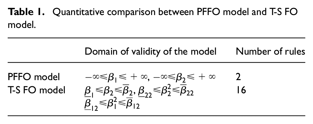
{\begin{matrix} _{0}^{C} D_{t}^{ς} β = \sum_{i = 1}^{2} δ_{i} {A_{i} (β) β + B_{i} (β) u} \\ y = C β \end{matrix}

(33)

Table 1 illustrates the main advantages of PFFO model compared with T-S FO model. The table indicates that utilizing fuzzy polynomial models leads to a decrease in the number of if-then rules, thereby reducing both the complexity and computation time.

Table 1.

Quantitative comparison between PFFO model and T-S FO model.

	Domain of validity of the model	Number of rules
PFFO model	$- \infty \leq β_{1} \leq + \infty$ , $- \infty \leq β_{2} \leq + \infty$	2
T-S FO model	${\underline{β}}_{1} \leq β_{2} \leq {\bar{β}}_{2}$ , ${\underline{β}}_{22} \leq β_{2}^{2} \leq {\bar{β}}_{22}$	16
	${\underline{β}}_{12} \leq β_{1}^{2} \leq {\bar{β}}_{12}$

Remark 4: The PFFO can reduce the number of rules required to describe the system, leading to a simpler and more interpretable model than the T-S fuzzy model. For example, the PFFO (33) can be represented by T-S FO model with 16 rules by posing $β_{1}^{2}$ , $β_{2}$ , and $β_{2}^{2}$ as premise variables.

Remark 5: Since $A_{1} (β)$ and $A_{2} (β)$ contain unmeasurable state $β_{2}$ . Then, all results in the literature related to observer-based control of T-S fuzzy model with measurable membership functions, using the linear matrix inequalities approach, cannot be applied.

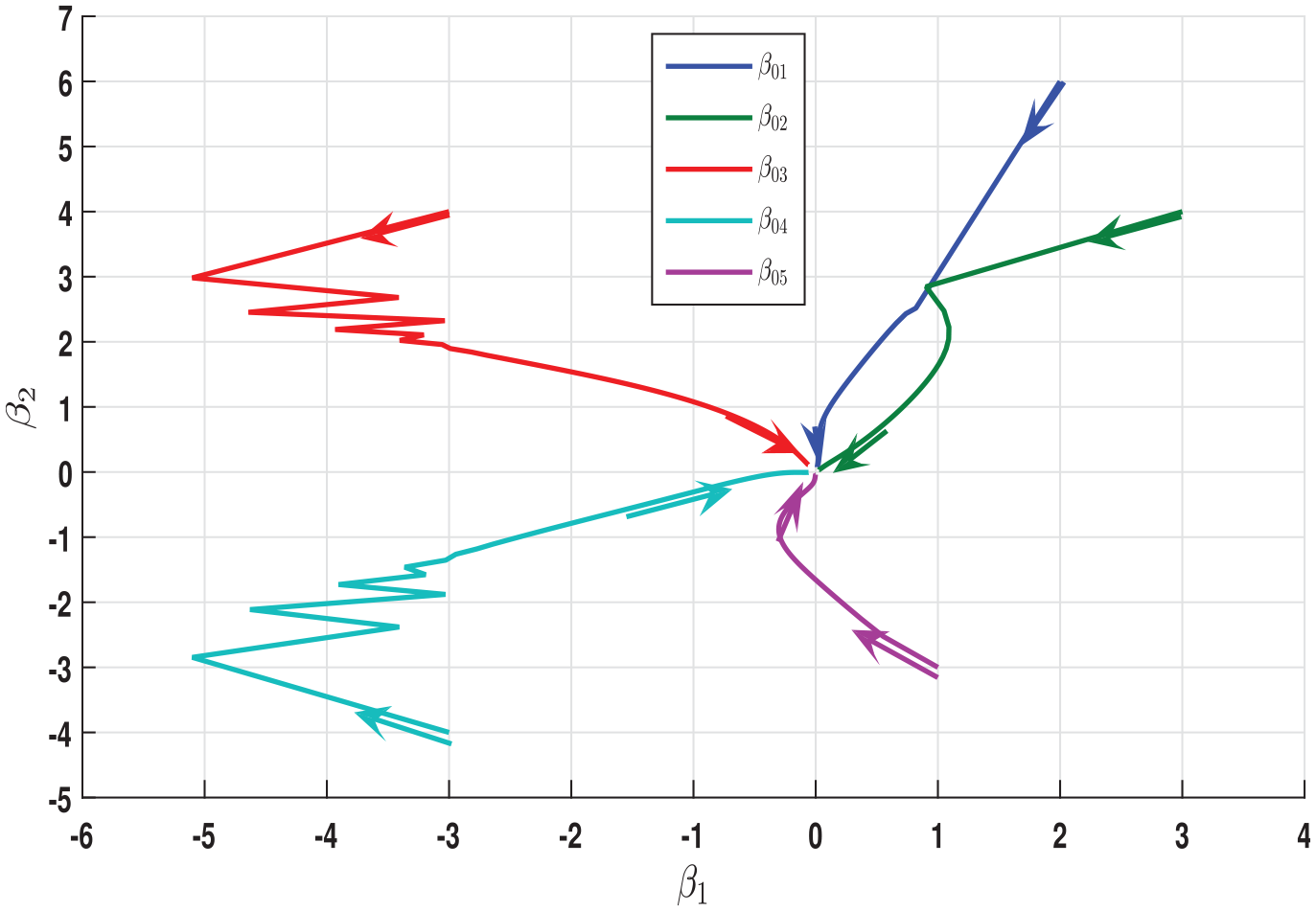
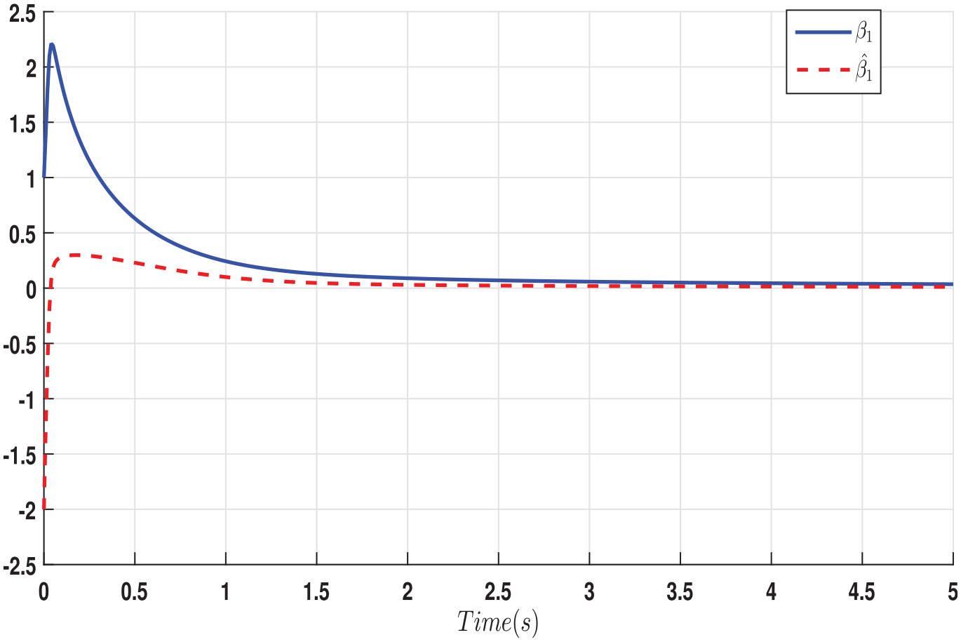
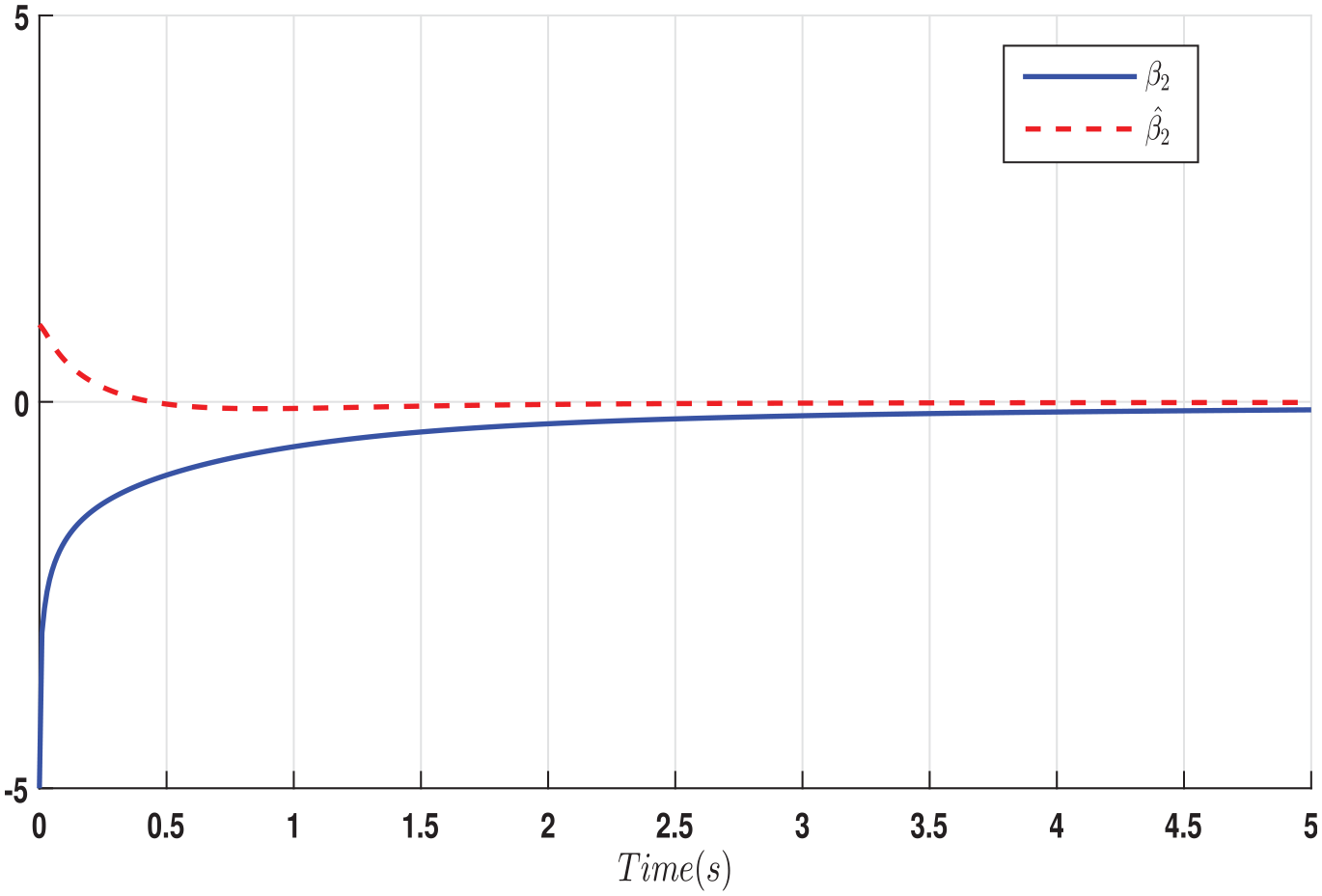
Remark 6: For simulation purposes, we have adapted the algorithms proposed in Vityuk and Mykhailenko (2011) and Arfaoui and Ben Makhlouf (2022).

Simulations results are presented in Figures 6 –9. Figure 6 shows the $β_{1} - β_{2}$ phase plane for PFFO model (33) with $u = 0$ for different initial conditions $β_{01} = [\begin{matrix} 2 & 6 \end{matrix}], β_{02} = [\begin{matrix} 3 & 4 \end{matrix}],$ $β_{03} = [\begin{matrix} - 3 & 4 \end{matrix}], β_{04} = [\begin{matrix} - 3 & - 4 \end{matrix}], β_{04} = [\begin{matrix} 1 & - 3 \end{matrix}]$ . Figure 7 shows the control trajectories of PFFO model (33) for the same initial states as in Figure 5. The system states $β$ and their estimation, for the initial conditions $β_{0} = [\begin{matrix} 1 - 5 \end{matrix}], {\hat{β}}_{0} = [\begin{matrix} - 2 1 \end{matrix}]$ , are illustrated in Figures 8 and 9.

Conclusion

This paper investigated the observer-based control problem for a class of PFFO model. The general case, in which the polynomial matrices depend not only on measurable states but also on unmeasurable states, is considered in this work. The dynamics of the PFFO model and the FO polynomial fuzzy observer-based controller are augmented to form the closed-loop system. By adopting the Lyapunov theory, two design procedures stability analysis for the developed augmented system are proposed. The first one is given in only one step involve three independent symbolic variables. However, the second one is presented in two steps involve two independent symbolic variables. A numerical example is given in order to demonstrate the importance of the reduction of the number of symbolic variables in SOS-based conditions. This allows us to reduce not only the conservatism but also the computational complexity. In a future work, we can extend our results by using another fractional derivative like Atangana–Baleanu fractional derivative.

Footnotes

Declaration of conflicting interests

The author(s) declared no potential conflicts of interest with respect to the research, authorship, and/or publication of this article.

Funding

The author(s) disclosed receipt of the following financial support for the research, authorship, and/or publication of this article: This research was funded by Researchers Supporting Project number (RSPD2023R683), King Saud University, Riyadh, Saudi Arabia.

ORCID iDs

Hassen Arfaoui

Abdellatif Ben Makhlouf

References

Alikhanov

(2010) A priori estimates for solutions of boundary value problems for fractional-order equations. Differential Equations 46: 660–666.

Arfaoui

Ben Makhlouf

(2022) Some results for a class of two-dimensional fractional hyperbolic differential systems with time delay. Journal of Applied Mathematics and Computing 68: 2389–2405.

Boulham

Boubakir

Labiod

(2023) Fuzzy

L_{1}

adaptive controller for chaos synchronization of uncertain fractional-order chaotic systems with input nonlinearities. Transactions of the Institute of Measurement and Control. Epub ahead of print 12 February. DOI: 10.1177/01423312221148241.

Chen

Zhang

, et al. (2016) New relaxed stability and stabilization conditions for continuous-time T-S fuzzy models. Information Sciences 329: 447–460.

Chibani

Chadli

Ding

, et al. (2018) Design of robust fuzzy fault detection filter for polynomial fuzzy systems with new finite frequency specifications. Automatica 93(1): 42–54.

Duan

(2018) Observer-based non-PDC controller design for T-S fuzzy systems with the fractional-order

α : 0 < α < 1

. IET Control Theory & Applications 12(5): 661–668.

Elias

Faria

Araujo

, et al. (2021) Stability analysis of Takagi-Sugeno systems using a switched fuzzy Lyapunov function. Information Sciences 543: 43–57.

Fan

Wang

(2022) A fuzzy Lyapunov function method to stability analysis of fractional-order T-S fuzzy systems. IEEE Transactions on Fuzzy Systems 30(7): 2769–2776.

Iben Ammar

Gassara

Hajjaji

, et al. (2021) DC-DC buck converter polynomial tracking control design with saturation constraint. In: 60th IEEE conference on decision and control (CDC), Austin, TX, 14–17 December.

10.

Kilbas

Srivastava

Trujillo

(2015) Theory and Application of Fractional Differential Equations. New York: Elsevier.

11.

Chen

Podlubny

(2009) Mittag-Leffler stability of fractional order nonlinear dynamic systems. Automatica 45: 1965–1969.

12.

Lin

Wang

Lee

(2005) Improvement on observer-based

H_{\infty}

control for T-S fuzzy systems. Automatica 41(9): 1651–1656.

13.

Liu

(2015) Design of a polynomial fuzzy observer controller with sampled-output measurements for nonlinear systems considering unmeasurable premise variables. IEEE Transactions on Fuzzy Systems 23(6): 2067–2079.

14.

Naifar

Ben Makhlouf

Hammami

, et al. (2018) Global practical Mittag-Leffler stabilization by output feedback for a class of nonlinear fractional-order systems. Asian Journal of Control 20(1): 599–607.

15.

Papachristodoulou

Anderson

Valmorbida

, et al. (2021) SOSTOOLS: Sum of squares optimization toolbox for MATLAB version 4.00. Available at: https://par.nsf.gov/biblio/10353822

16.

Podlubny

(1999) Fractional Differential Equations. San Diego, CA: Academic Press.

17.

Takagi

Sugeno

(1985) Fuzzy identification of systems and its applications to modeling and control. IEEE Transactions on Systems, Man and Cybernetics 15(1): 116–132.

18.

Tanaka

Ohtake

Seo

, et al. (2012) Polynomial fuzzy observer designs: A sum-of-squares approach. IEEE Transactions on Fuzzy Systems 42(5): 1330–1342.

19.

Tanaka

Yoshida

Ohtake

, et al. (2009) A sum-of-squares approach to modeling and control of nonlinear dynamical systems with polynomial fuzzy systems. IEEE Transactions on Fuzzy Systems 17(4): 911–922.

20.

Vityuk

Mykhailenko

(2011) The Darboux problem for an implicit fractional-order differential equation. Journal of Mathematical Sciences 175: 391–401.