
Abstract
In this paper, we present an innovative approach for assessing the stability of linear time-invariant (LTI) systems. The key innovations in our methodology include the calculation of Markov parameters, the extension to nonlinear continuous-time systems, and significantly improved computational efficiency. Our novel approach leverages Markov parameters derived from the characteristic polynomial of the system. Unlike traditional methods, we employ the Leverrier-Takeno algorithm to efficiently determine the coefficients of the characteristic polynomial for state-space representation. The systematic calculation of Markov parameters using a specialized Maclaurin series expansion enhances our method’s precision. One of our major achievements is the rigorous verification of stability through Hankel matrices, ensuring positive definiteness using the Cholesky decomposition algorithm. In addition, we introduce a second stability criterion based on iterated polynomial long divisions, although we acknowledge its limitations in handling high-order systems due to computational inefficiency. Our pioneering contributions extend beyond LTI systems. We adapt our innovative techniques to analyze the local stability of nonlinear continuous-time systems by introducing the concept of Jacobian matrices and employing the indirect Lyapunov method. This expansion broadens the applicability of our approach to a wider range of real-world systems. Notably, our approach exhibits remarkable computational efficiency. According to CPU-time analysis, our first stability criterion outperforms the classical Routh–Hurwitz method by more than 12 times for dynamic systems with orders ranging from 2 to 180. This significant reduction in computation time positions our method as a valuable option for real-time stability analysis applications.
Keywords
Introduction
The stability of control systems is a crucial property that affects their performance, safety, and reliability. Therefore, a considerable amount of control engineering literature deals with the principles and techniques for assessing different stability definitions. The bounded-input-bounded-output (BIBO) stability is one of these concepts that plays a key role in the design and analysis of control systems. It ensures that the dynamic system will behave predictably and will not exhibit any unexpected behavior (Corriou, 2013). In fact, the nature of the roots of the characteristic polynomial associated with a system dictates its BIBO stability. If all the mentioned roots have negative real parts, the BIBO stability of the system is guaranteed. However, it is naïve and simplistic to solely rely on calculating the characteristic polynomial roots to determine a system’s stability because (a) there is no exact algebraic root-finding technique for polynomial equations of order five or higher, according to the Abel–Ruffini theorem, aka the “impossibility theorem,” (b) even using numerical root-finding algorithms, the results will sometimes suffer from large magnitudes of error if the polynomial is ill-conditioned (Cheney and Kincaid, 2009; Cohen, 1994).
Consequently, several stability assessment methods have been developed, which are based on identifying the regional location of the characteristic roots in the complex plane rather than their exact values. Examples of such methods are the Hurwitz criterion, the Routh–Hurwitz method, and Evans root locus method. Unfortunately, each of these methods has their own drawbacks. For instance, the Hurwitz and the Routh–Hurwitz methods are only applicable to real characteristic polynomials. They also cannot handle systems whose closed-loop transfer function includes non-algebraic terms, such as time delays. Furthermore, both methods are inefficient for higher-order systems from a computational viewpoint. The Evans root locus method is not applicable to multi-input-multi-output (MIMO) systems and cannot be applied to time-varying models. It can be time-consuming as a graphical method, especially for complicated higher-order systems and it does not account for time delays (Abolpour et al., 2023; Cogan et al., 2009; Fatoorehchi and Djilali, 2023; Kavitha and Ramakalyan, 2014; Shinskey, 1996). It is worthwhile to mention that Yang et al. (2022) have generalized the Routh–Hurwitz technique to fractional-order linear systems, and their method is called the fractional-order Routh–Hurwitz stability criterion.
The most recent BIBO stability criterion for LTI systems is an integrative method that is founded on an efficient approach for computing the Bézoutian matrix associated with the system under investigation, aiming subsequently to derive the system’s Hermite–Fujiwara matrix (Fatoorehchi and Ehrhardt, 2023).
Table 1 provides a brief overview of the advantages and drawbacks of the conventional stability criteria, facilitating quick comparison.
Comparison of stability analysis methods.
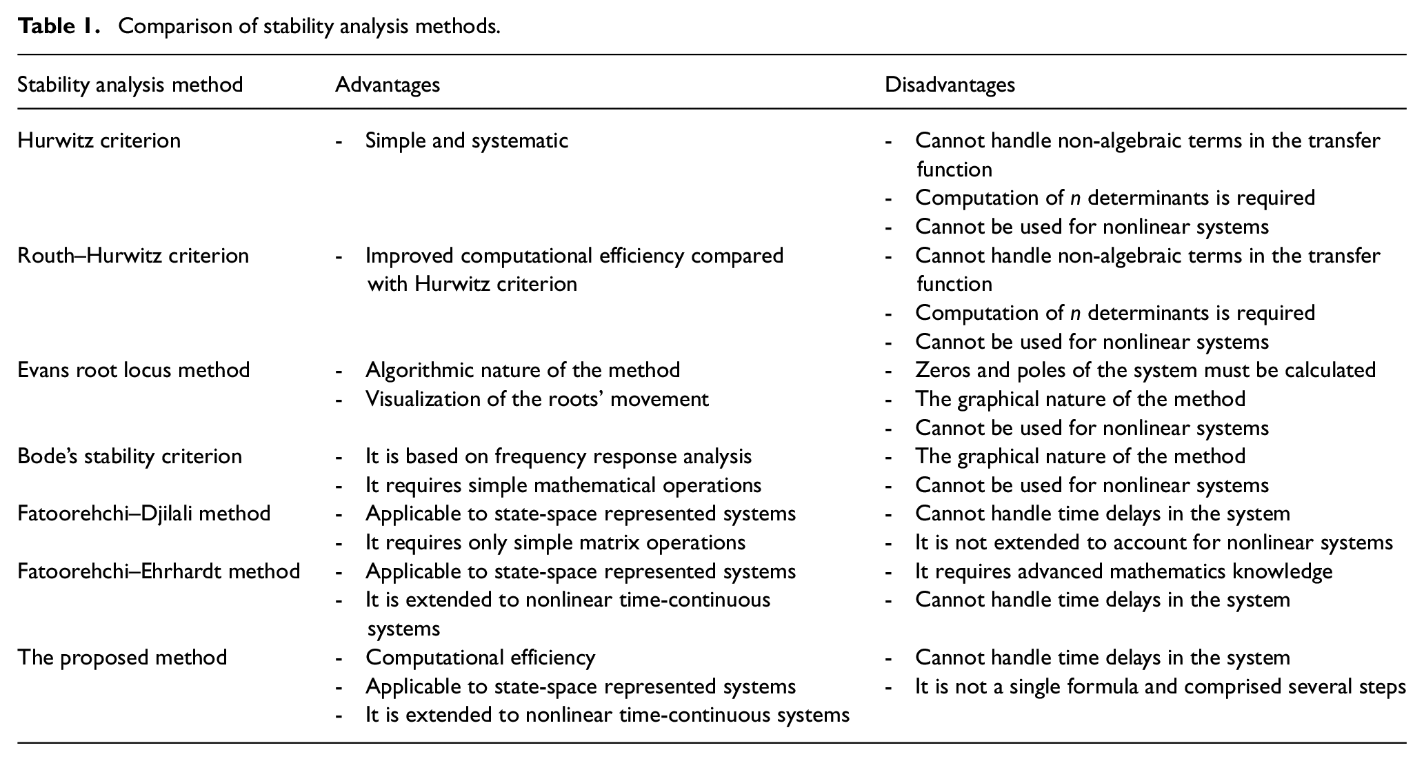
It should be noted that fast or real-time stability analysis is particularly favored in practice for several industries. For these applications, the computationally efficient stability criteria are often preferred over more complex methods that require significant computational resources and time efforts. For instance, real-time stability assessment of power grid systems, with a typical frequency of 10 Hz, is essential to a transient-free power management. Furthermore, very fast stability analyses are required to control intensified unit operations of chemical engineering, such as spinning disk reactors or multiloop chemical reactors (Ghiasy et al., 2012; Sun et al., 2016; Yakhnin and Menzinger, 2004).
In this paper, we will develop a novel stability criterion for linear time-invariant (LTI) systems by exploiting the Maclaurin series expansion for evaluating the Markov parameters of rational functions. In the course of our algorithm, we will take benefit from the Leverrier-Takeno algorithm for calculating the characteristic polynomial, if the system is given in the state-space form, and the Cholesky decomposition for checking positive definiteness of the associated Hankel matrices. We will demonstrate that our approach is computationally efficient and valid for MIMO systems. A set of case studies involving distillation columns and a nonlinear boiler-turbine unit is given to demonstrate the methodology and application of our proposed method.
Mathematical background
In this section, we present the mathematical background that serves as the foundation for the methodology described in the subsequent section. Specifically, we introduce the necessary definitions and theorems. By laying out this mathematical background, we aim to provide a comprehensive and self-contained exposition of our approach, that is accessible for a broad audience.
Furthermore, let
Methodology overview
Let the characteristic polynomial associated with the system matrix

We define the rational function
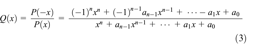
The Markov parameters associated with the rational function
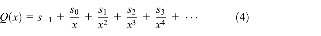
where the convergence of the right-hand side of equation (4) does not play a role in defining
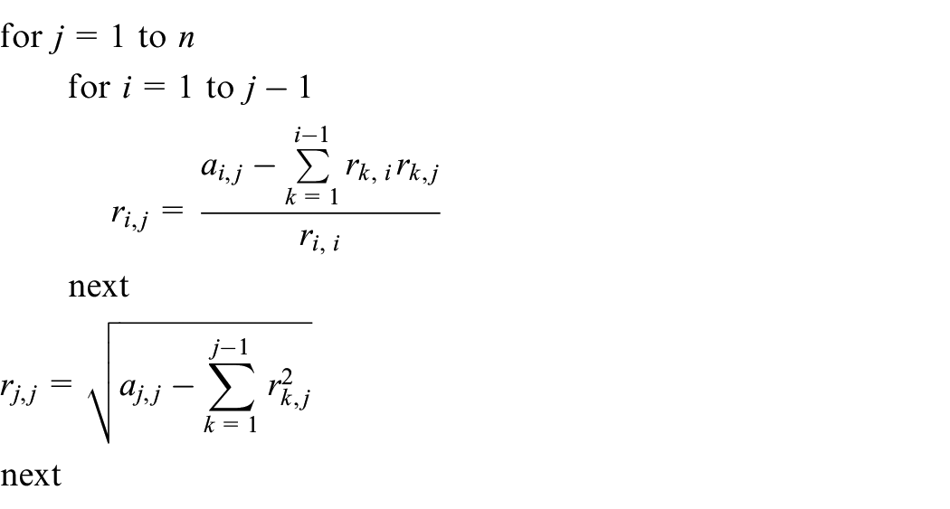
For calculation of the Markov parameters, we will take advantage of the Maclaurin expansion. To do so, let us assume that the function
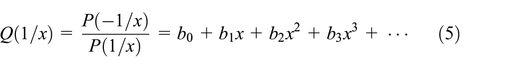
Next, by a simple reciprocal variable change, we can deduce that
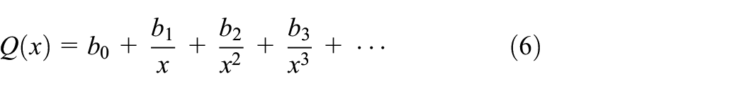
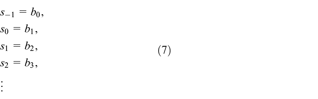
If we compare equations (4) and (6), then we readily obtain the Markov parameters of the rational function
Subsequently, with the help of the Markov parameters, we can formally define the infinite Hankel matrix as
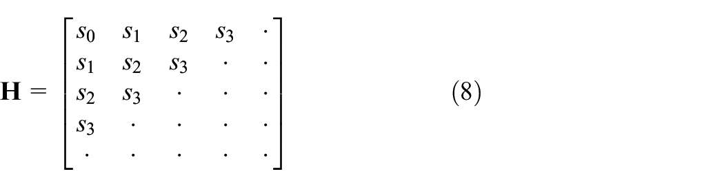
It is clear from equation (8) that each Markov parameter fills an anti-diagonal of the infinite Hankel matrix.
Next, we define the submatrix
such that
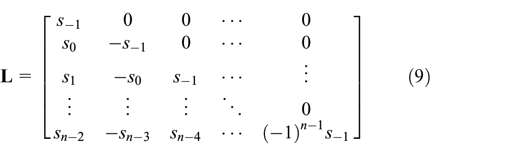
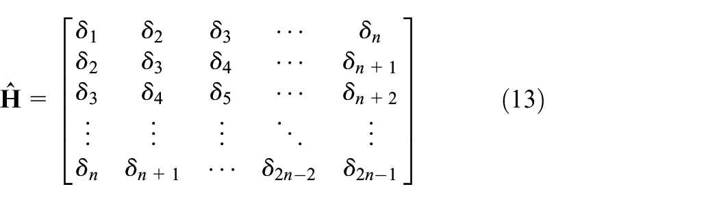
Finally, we introduce the matrix

by which the stability of the system under study can be assessed according to the subsequent theorem.
Considering equations (8)–(10), it is important to underscore that our stability criterion relies solely on the first n Markov parameters, indicating that the subsequent Markov parameters (beyond the nth) hold no significance in the stability status of the studied system.
Another stability criterion can be formulated based on a distinct set of Markov parameters and an alternative definition of the Hankel matrix (see Theorem 3.2).
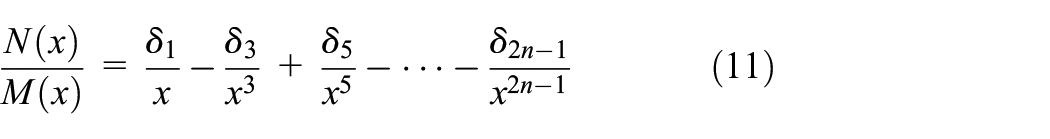
and if n is odd, then we construct the following expansion
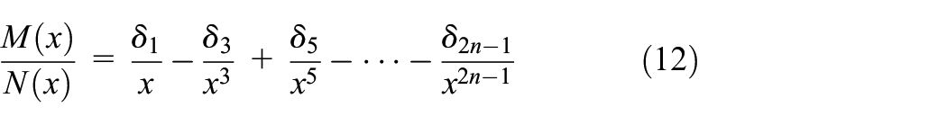
where
Now, the system characterized by
Note that the expansions in the right-hand sides of equations (11) and (12) should be derived from repeated polynomial long divisions, which is a time-intensive and tedious task especially for higher-order systems. Thus, we use Corollary 3.2 as our second stability criterion only for systems with a small number of state functions in the next section and rely on Corollary 3.1 as our main stability test.
In the end of this section, we emphasize that our stability criteria can be extended to nonlinear continuous-time systems for local stability analysis by replacing the state matrix

such that

and also, let
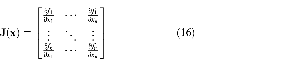
It holds that if all eigenvalues of matrix

whose equilibrium point is different from that of equation (14) and actually is transferred from
For better illustration, the flowchart of our first and second stability criteria, the ones based on Corollary 3.1 and 3.2, is depicted in Figures 1 and 2.
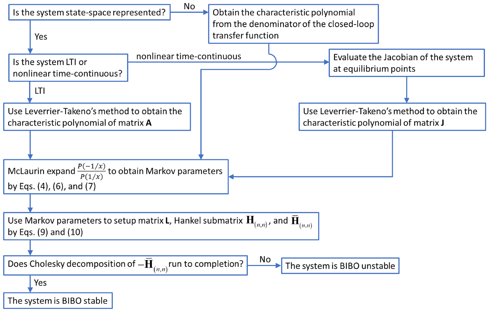
Flowchart of the first proposed stability criterion (Corollary 3.1).
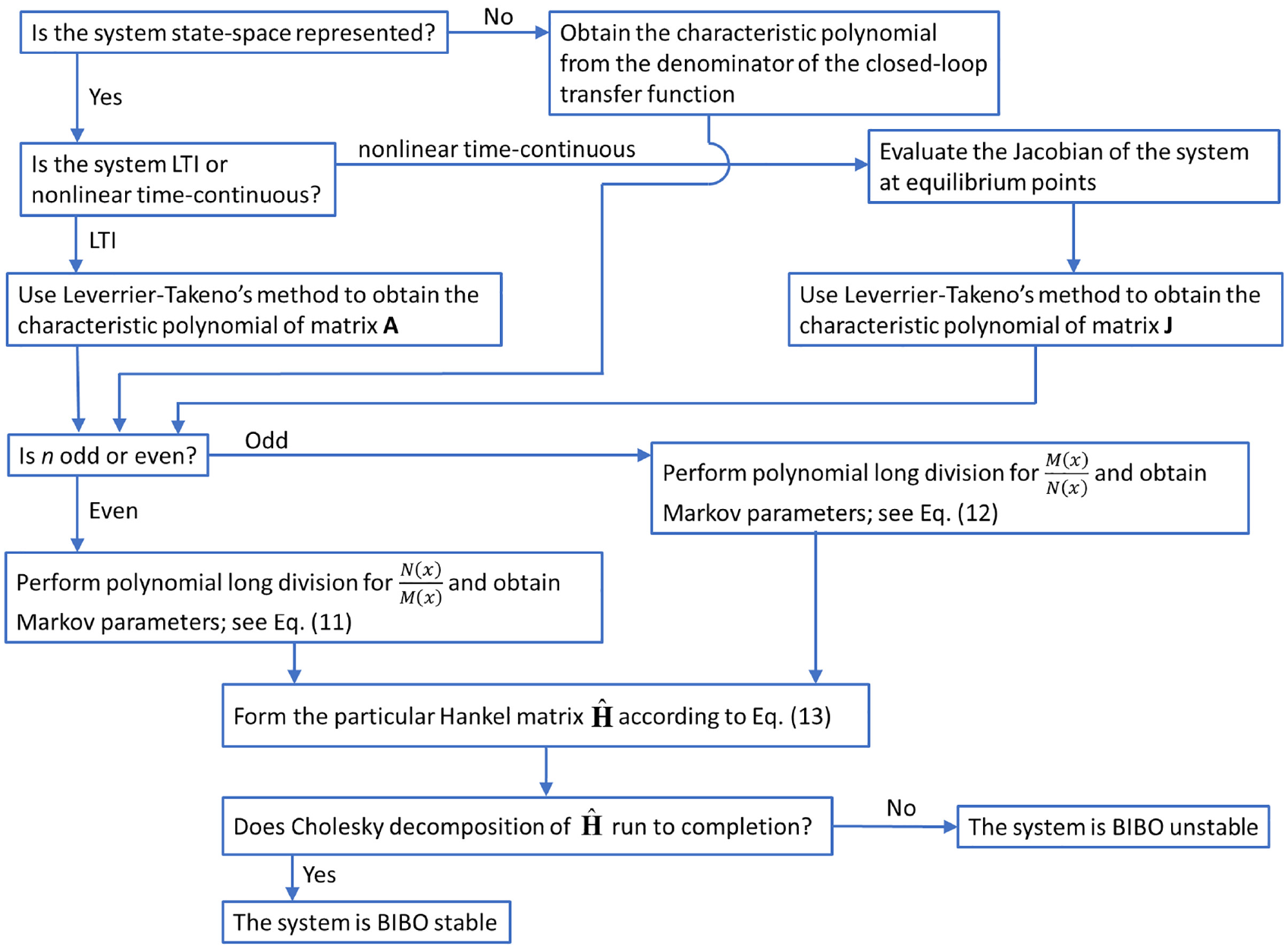
Flowchart of the second proposed stability criterion (Corollary 3.2).
Illustrative examples
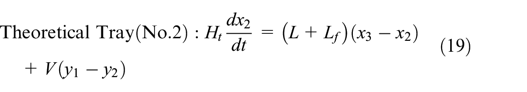
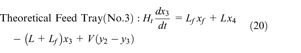
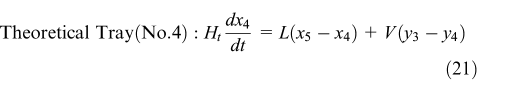
Example 1. Binary distillation column with three trays
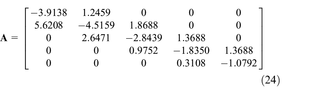
Rasmussen and Jørgensen (1999) modeled a binary distillation column comprising a total condenser, a reboiler, and three equilibrium (theoretical) trays. The dynamics of the column is governed by a system of five nonlinear ordinanry differential equations (ODEs) that are derived from appropriate mole balances


in which molar compositions of the liquid and vapor phases in the trays and the reboiler are subject to thermodynamic equilibrium simplistically modeled by
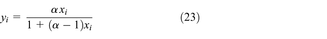
where
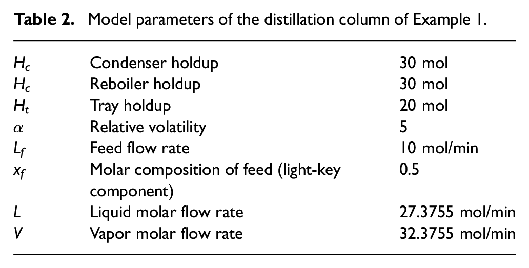
Model parameters of the distillation column of Example 1.
We examine the stability of the system at such operating conditions subsequently.
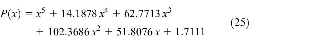
Using the Leverrier-Takeno method (Theorem 2.2), we derive the characteristic polynomial as
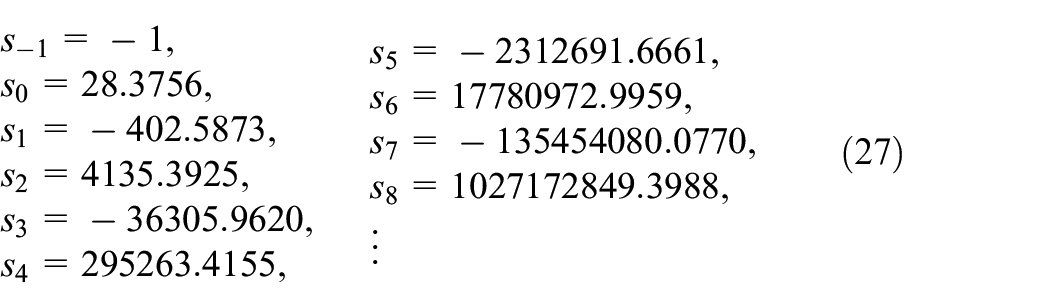
Expanding the function

In view of equations (5), (7), and (26), we identify the Markov parameters of
Afterward, the infinite Hankel matrix is formally constructed as
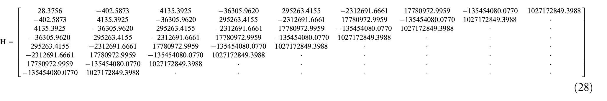
and from which the submatrix
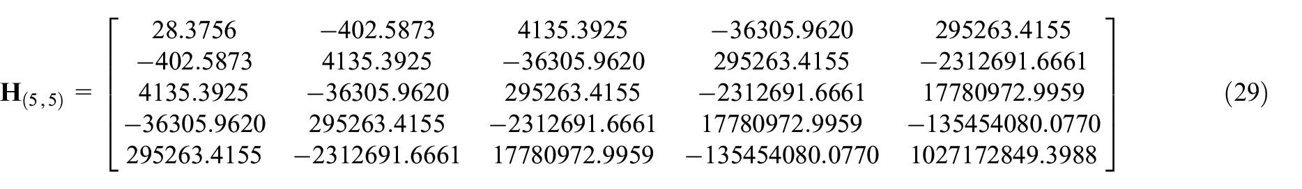
Then, we define matrix
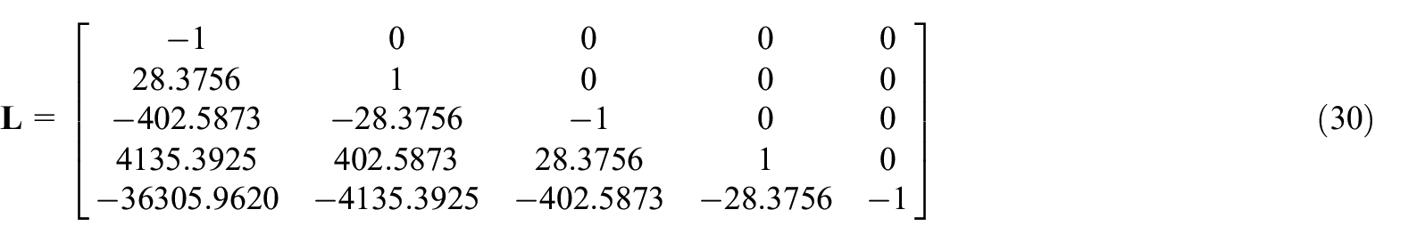
Finally, by means of equation (10), we calculate matrix
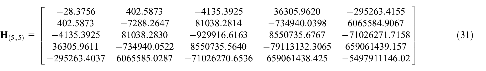
Note that the calculated
Subsequently, we try the Cholesky decomposition algorithm on the matrix
Since all diagonal entries
Now, we will examine the stability of the system by the second approach, that is, Corollary 3.2.
In view of Theorem 3.2 and equation (12), it is clear that we have to expand

and

After a series of polynomial long divisions, we will derive the following nine Markov parameters according to equation (12)
Afterward, the relevant Hankel matrix is derived as
Following that, we try the Cholesky decomposition algorithm on matrix
The fact that all the diagonal components are real, shows that the Cholesky algorithm has run to completion and thus, matrix
Example 2. Binary distillation column with eight trays
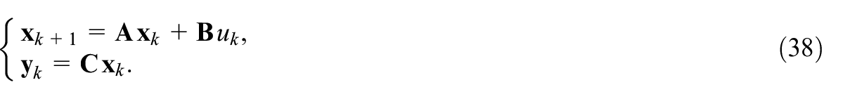
Drgoňa et al. (2017) developed a data-driven model for a laboratory distillation column as depicted in Figure 3 for separating methanol and water. The column consisted of eight sieve trays, a reboiler, and a total condenser. An LTI model in the discrete domain was constructed by exerting a sufficient number of inputs to the experimental system and collecting the output responses. The model is expressed as
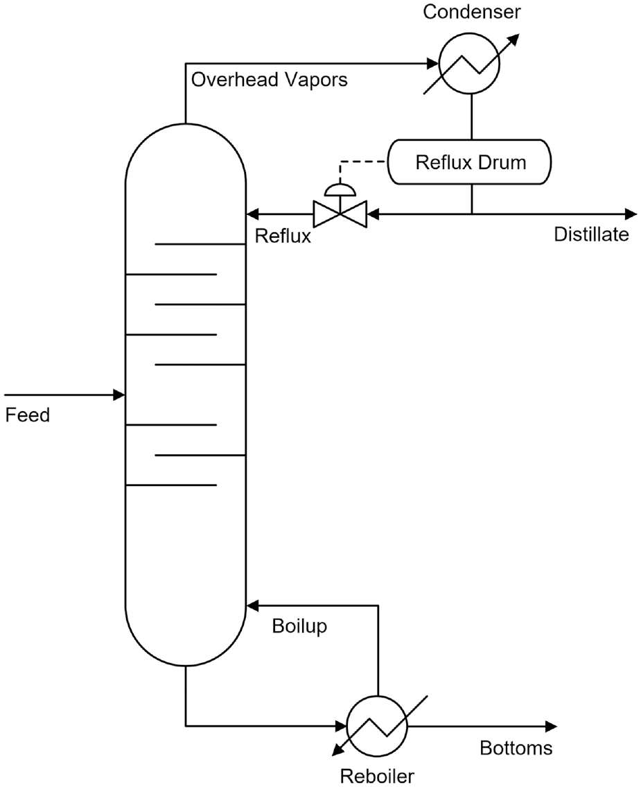
Schematic view of the distillation column of Example 2.
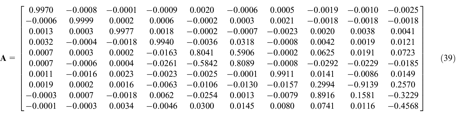
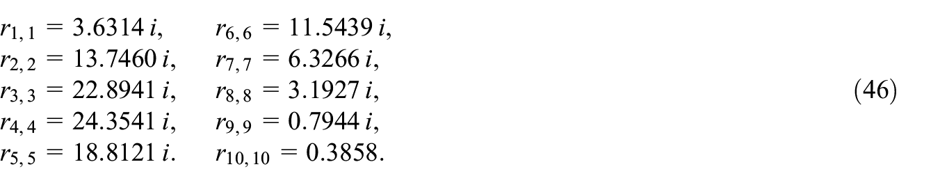
The system matrix for the dynamics of the distillation column at a particular operation point is
The characteristic polynomial of the matrix

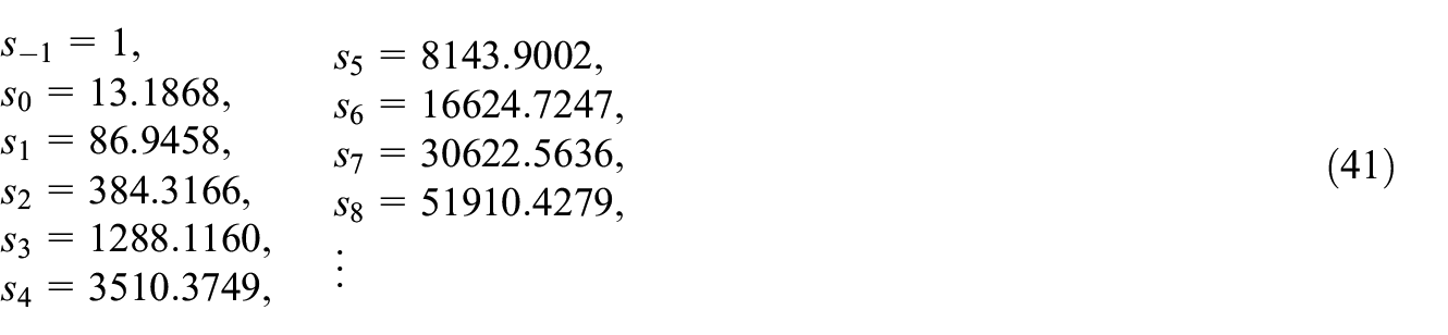
To streamline the presentation, here we will skip some of the less crucial steps that were demonstrated in the previous example and list the related Markov parameters as
Thus, the infinite Hankel matrix is formally determined accordingly
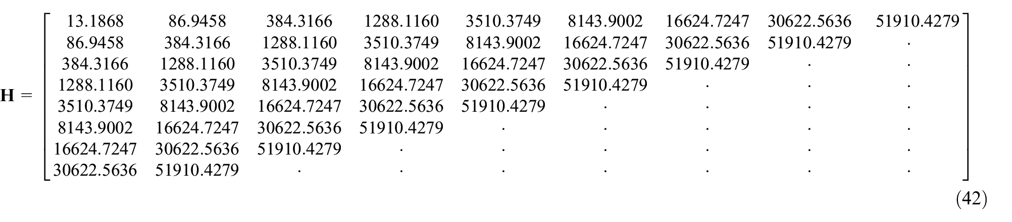
Then, it is straightforward to generate the submatrix
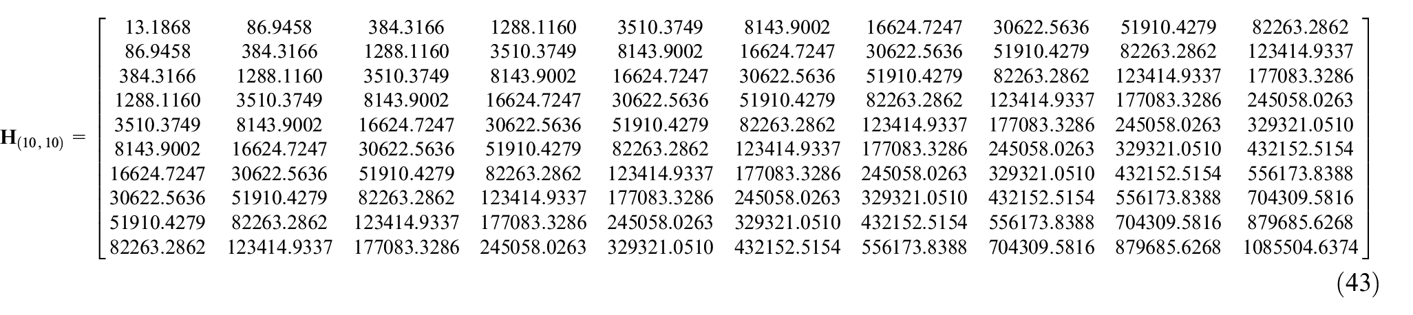
The next leading step is to compute the
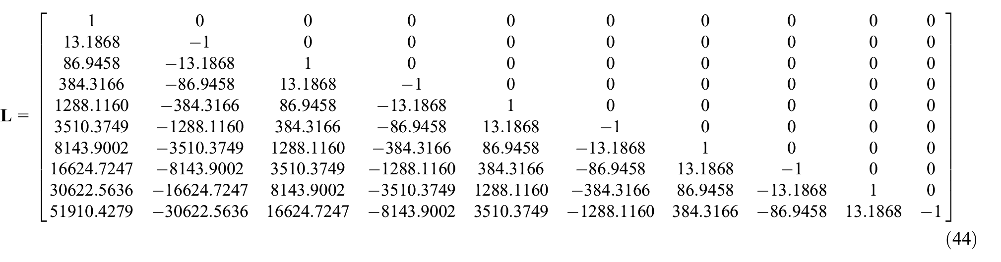
Afterward, we construct
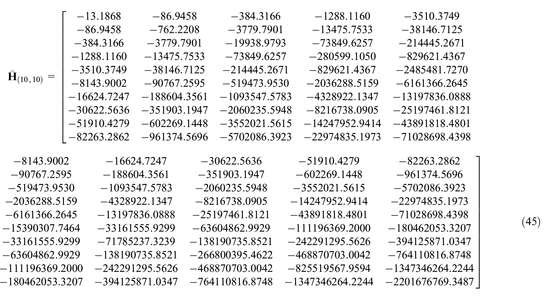
Finally, we apply the Cholesky decomposition on
Since there are non-real entries on the diagonal of the matrix
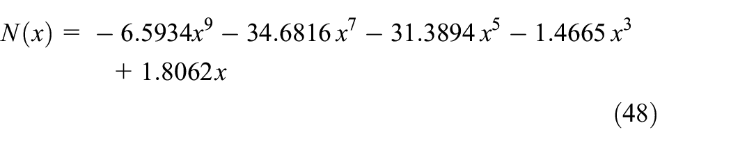
Let us now apply the second stability test outlined in Corollary 3.2 to system (38). As the characteristic polynomial equation (40) is even-ordered, we should expand the rational function
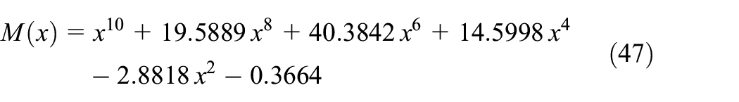
and
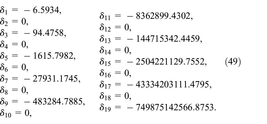
After repetitive polynomial long divisions, the 19 Markov parameters are read according to equation (11)
Next, the Hankel matrix
On Cholesky decomposition, we notice that the matrix
As a result, system (38) at the given conditions cannot be stable.
Example 3. A hypothetical 13th-order system
As a demanding benchmark, we will test our method for a stable, hypothetical system with 13 states. The order of the system is high enough to be a fair representative of many chemical engineering unit operations. The characteristic polynomial of this system in the product form is
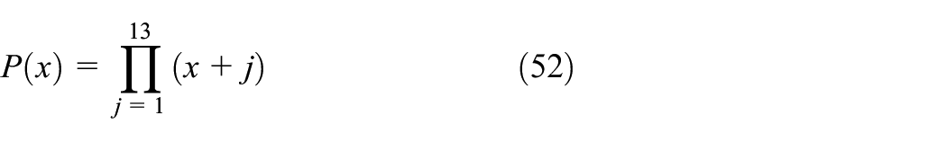
We can invoke Vieta’s formulas to determine the coefficients of our characteristic polynomial as follows
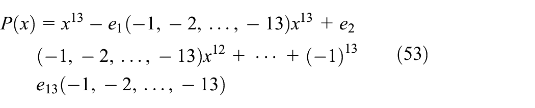
where e denotes elementary symmetric polynomials. Obviously, the system is stable as the roots of the characteristic equation, namely {–1, –2, –3, –4, –5, –6, –7, –8, –9, –10, –11, –12, –13}, all have negative real parts.
Skipping the less important steps in our procedure, we perform the Maclaurin expansion on the rational function
In the interest of brevity, we will omit several intermediate steps in the procedure again. Therefore, the diagonal entries of the upper triangular Cholesky factor of
As all the
Example 4. A nonlinear boiler-turbine system
The dynamics of a boiler-turbine unit has been modeled as the following system of ODEs (Tan et al., 2005)
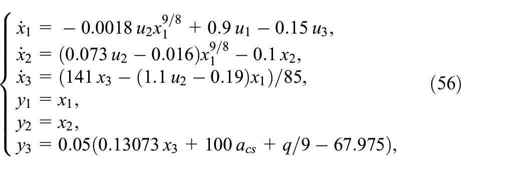
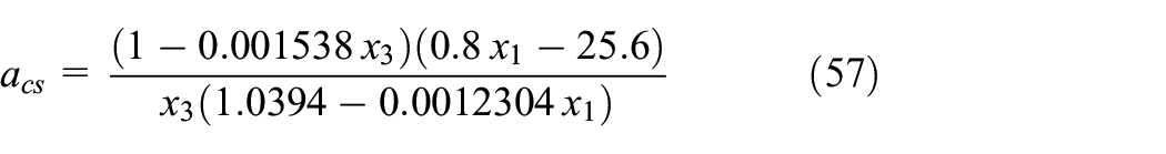
where the three state variables namely x1, x2, and x3 denote drum pressure (kg/cm2), electric power output (MW), and fluid density (kg/m3), respectively. The three inputs u1, u2, and u3 are the valve positions for the fuel, the steam, and the feed stream. The system’s output y3 is the drum water level (m). The parameters acs and q are the steam quality and the evaporation rate (kg/s), which are given by

It is clear that system (56) is MIMO and still our criterion is valid to analyze its stability.
We want to investigate the stability of system (56) at a particular steady-state condition (equilibrium point), namely
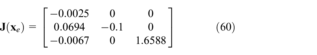
As the first step, we derive the Jacobian matrix associated with system (56) as
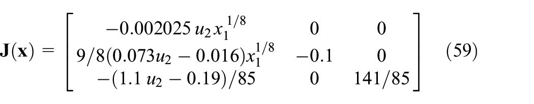
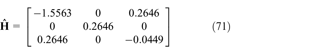
which is evaluated at the aforementioned equilibrium point as
Next, it is straightforward to obtain the characteristic polynomial of matrix

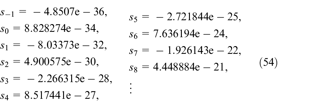
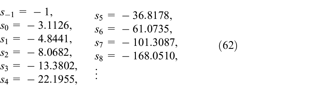
Subsequently, by a Maclaurin expansion of
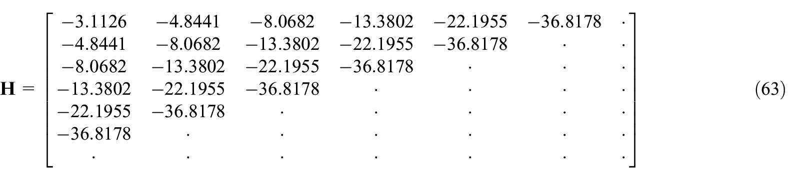
Then, the associated infinite Hankel matrix formally reads
and its submatrix
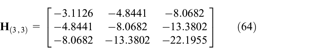
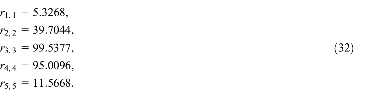
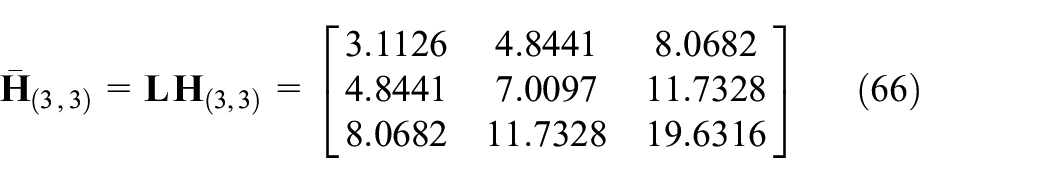
As the next step, the lower triangular matrix
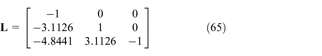
and immediately it follows that
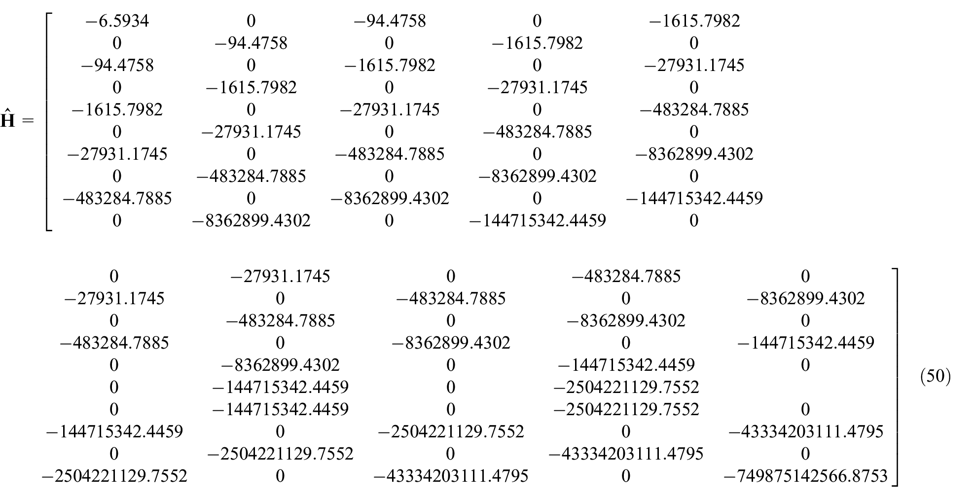
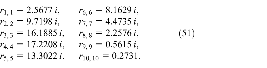
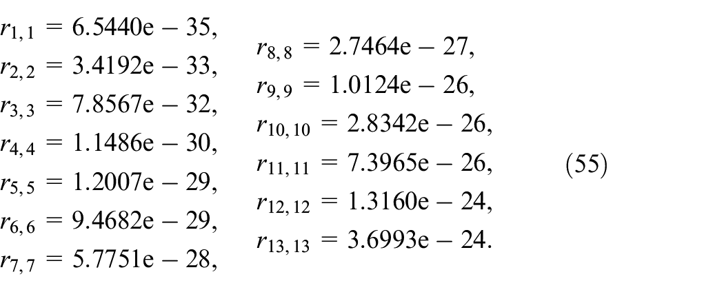
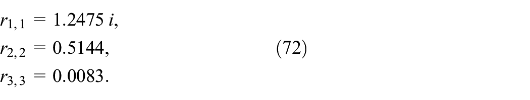
Finally, we perform the Cholesky decomposition on the matrix
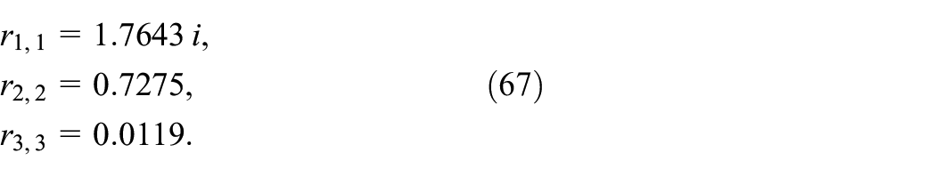
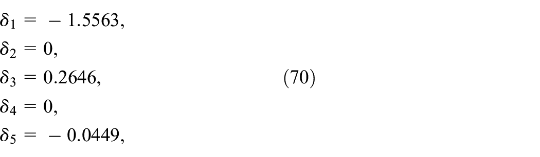
Since at least one diagonal component, that is
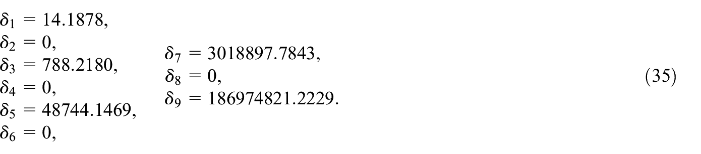
Alternatively, we will test our second criterion, namely Corollary 3.2 for system (56) in the sequel. From equation (61) it is easy to identify


Since the order of the characteristic polynomial, see equation (61), is odd, we understand that we must expand
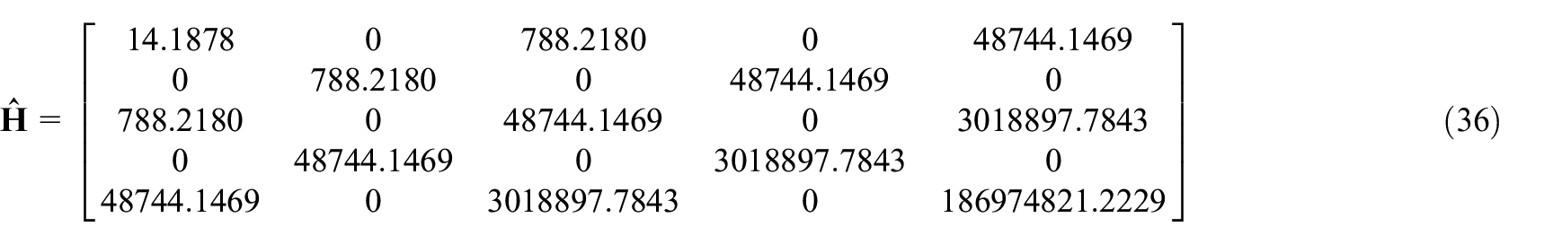
and from them, we build the Hankel matrix
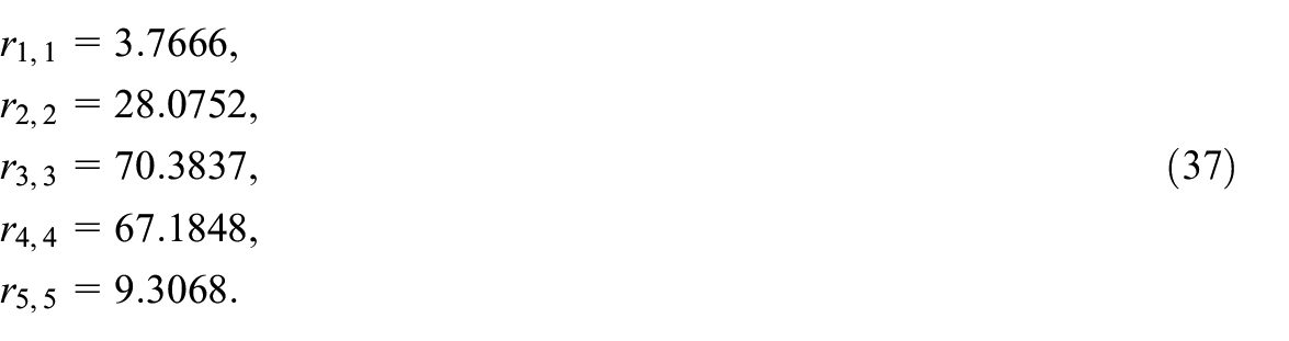
Afterward, we run a Cholesky decomposition to check the positive definiteness of matrix
The existence of a non-real entry in
Computational performance analysis
In this section, we will compare the computational performance of our first stability criterion, namely Corollary 3.1, against that of the Routh–Hurwitz method through a CPU-time benchmarking experiment on a set of randomly generated LTI dynamic systems with orders ranging from 2 to 180. The results of this comparative investigation are depicted in Figure 4 (observe the log-scale). Based on the average CPU-time values, we can conclude that our stability analysis algorithm is approximately 12.8 times faster than the Routh–Hurwitz method. This superiority can be attributed to the fact that the most time-consuming step in our approach is the Maclaurin expansion. The rest are simple substitutions and finally, a single matrix multiplication exists. In contrast, the Routh–Hurwitz algorithm entails a large number of arithmetic operations including multiplication, division, and subtraction for the completion of the Routh table prior to reaching a conclusion on the stability of the system under study. As a side note, we may even increase the computational speed of our method for some cases by exploiting the fact that on the appearance of a non-real diagonal entry in the Cholesky pseudo code, see Definition 2.4, we can prematurely terminate the algorithm in favor of computational efficiency and conclude unstability.
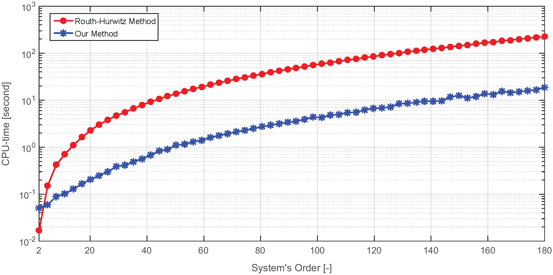
Computational efficiency analysis of our stability criterion and the Routh–Hurwitz method.
Moreover, in contrast to the Routh–Hurwitz method, which has certain special cases that require special handling and can significantly impact computational performance, our proposed stability criterion is free of such exceptions. These special cases in the Routh–Hurwitz method, such as zero rows or columns in the Routh table, can lead to difficulties in determining the stability of a system and may require additional calculations or adjustments to account for their presence, resulting in increased computational complexity and time.
Our criterion, however, does not suffer from any such issues, as it is applicable to a wide range of linear control systems without the need for any special treatment or exceptions, and therefore offers a more reliable and efficient approach for stability analysis, particularly in terms of computational performance, when compared to the Routh–Hurwitz method and its special cases.
Conclusion
We developed a stability criterion for LTI systems based on Markov parameters of a rational function that is defined from the characteristic polynomial of the system under study. For state-space represented dynamic systems, we used the Leverrier-Takeno algorithm to derive the coefficients of the characteristic polynomial as the initial step. Afterward, the Markov parameters were systematically calculated by a particular Maclaurin series expansion. The relevant Hankel matrices were then generated. The positive definiteness of the appropriate Hankel matrix was verified by the Cholesky decomposition algorithm as the final step of our criterion.
Furthermore, a second criterion was also developed that extracted a different set of Markov parameters of a distinct rational function from the characteristic polynomial by iterated polynomial long divisions. The latter was concluded to be computationally inferior as it entails repeated time-consuming polynomial long divisions. Hence, it was suggested suitable only for low-ordered systems.
Our methods were extended for the local stability analysis of nonlinear continuous-time systems by the concept of the Jacobian matrix and the indirect Lyapunov method of stability. The application of the proposed stability criteria was demonstrated through four illustrative examples including two distillation columns and a nonlinear boiler-turbine combination. In the end, based on the conducted CPU-time analysis for dynamic systems with orders ranging from 2 to 180, it was revealed that our first stability criterion is about 12 times faster than the classical Routh–Hurwitz method. Hence, it can possibly be implemented in fast or real-time stability analysis schemes.
As highlighted within the “Introduction,” our stability criterion is constrained by its inability to accommodate systems with time delays. Nonetheless, it is worth noting that this limitation is a common characteristic shared by the majority of previously established methods, as demonstrated in Table 1.
We intend to improve the computational efficiency of our current method by employing a more advanced positive definiteness checking algorithm as developed by Rump (2006), in a future research work.
Footnotes
Acknowledgements
The authors thank the editor and reviewers of the Transactions of the Institute of Measurement and Control for their invaluable comments and suggestions, which have significantly enhanced the quality of this paper. In addition, the first author (H.F.) thanks Raybod Fatoorehchi for diligently proofreading the paper drafts.
Declaration of conflicting interests
The author(s) declared no potential conflicts of interest with respect to the research, authorship, and/or publication of this article.
Funding
The author(s) received no financial support for the research, authorship, and/or publication of this article.