
Abstract
The goal of this research was to quantify the mobility and safety impacts of different combinations of lane width and shy distance to the barrier for a given paved width in work zones. The research team developed a device to measure lateral distance and derive speed, vehicle length/type, and headway information under day and night conditions. Data were collected at 17 locations in Illinois, Michigan, and Wisconsin. Lateral distance data of over a quarter million vehicles were used for the safety analysis. Extreme value theory modeling was conducted to estimate the probabilities of right-hand edge line encroachment and right-hand barrier contact. Wider lanes were found to have decreased probabilities of edge line encroachment and barrier contact, while wider shy distances were associated with increased probability of edge line encroachment and decreased probability of barrier contact. The speeds of over 125,000 free flow vehicles were used to quantify the mobility impact. Linear regression was implemented to develop models for estimating free flow speeds in work zones. Work zone free flow speed increased with an increase in speed limit, lane width, and left-/right-hand shy distance to the barrier. A case study of a 55-mph posted work zone with two open lanes and barrier on both sides with 26-ft available paved width is presented. Results of the case study indicate that 11-ft lanes with 2-ft shy distance have a slightly lower probability of right-hand barrier contact (for vehicles in the right-hand lane) than 12-ft lanes with 1-ft shy distance, while having a greater free flow speed. This research has demonstrated how lateral distance can be collected and modeled along with speed data to assess safety and mobility impacts in work zones.
Keywords
Aging infrastructure and increasing traffic volumes necessitate extensive work zones on the highway system. According to the National Work Zone Safety Information Clearinghouse, in 2021, 956 fatalities, about 42,000 injuries, and about 106,000 crashes occurred in work zones in the U.S.A. ( 1 ). Work zones need to be designed within a given roadway paved width. This is especially the case with counter-directional flow when traffic is crossed over to opposing lanes. The challenge faced by designers is in understanding the safety and mobility implications of the allocation of lane width and shoulder width (or shy distances to barriers) for a given paved width. For example, if a paved width of 26 ft were available, would it be better to have two 12-ft lanes with 1-ft shoulder/shy distance or two 11-ft lanes with a 2-ft shoulder/shy distance? No past study has evaluated the safety and mobility impacts of combinations of lane widths and shoulder widths in work zones. The objective of this research was to quantify the work zone safety and mobility impacts of different combinations of lane widths and shy distances to the barrier for a given paved width. The second section provides a review of state practices and a summary of past research. The third section describes the data collection device and the sites where data were collected. The fourth and fifth sections present the safety and mobility analysis and modeling, respectively. The sixth section provides a case study illustrating how the models can be used and the seventh section presents the conclusions, limitations, and recommendations.
Literature Review
The authors conducted a literature review to document existing knowledge of the impacts of lane and shoulder widths on work zone mobility and safety. The following sections describe state practices, mobility impacts, and safety impacts.
State Practices
National Cooperative Highway Research Program (NCHRP) Report 581 documented state work zone design guidance and reported that states require or generally use 11 ft for lane width on freeways/high-speed highways while permitting 10-ft lanes under some circumstances ( 2 ). The American Association of State Highway and Transportation Officials (AASHTO) Green Book recommends a 2-ft offset be provided where a roadside barrier, wall, or other vertical element adjoins shoulders ( 3 ). The Roadside Design Guide, Chapter 9, also recommends a 2-ft offset to portable concrete barriers ( 4 ). According to NCHRP Report 581, “The DOTs [departments of transportation] of Alabama, Missouri and Nevada strive to offset barriers 2 ft from the traveled way. Virginia DOT reported that barriers are normally placed from 0.5 to 1 ft from the traveled way edge lines” ( 2 ). The research team learned from conversations with work zone engineers in Michigan and Wisconsin that the general practice is to have the barriers at 2-ft offset in their states.
Mobility Impacts
Limited research has been conducted on the impact of lane and shoulder widths on speeds of vehicles in work zones. Chitturi and Benekohal ( 5 ) examined the impact of lane and shoulder widths on speeds using field data from 11 work zones in Illinois. The reductions in free flow speeds of vehicles in work zones because of narrow lanes were higher than the reductions given in the Highway Capacity Manual (HCM) for basic freeway sections. The narrower the lane, the greater the speed reduction, and the reduction in the free flow speeds of heavy vehicles was greater than the reduction in the free flow speeds of passenger cars. The HCM, 7th Edition, includes a formula for estimating the free flow speed in work zones ( 6 ). However, this formula does not account for lane or shoulder widths. The factors considered are the work zone speed limit, ratio of work zone speed limit to non-work zone speed limit, lane closure severity, barrier type, day/night, and number of on/off ramps. Edara et al. ( 7 ) modeled the impact of work activity on speed and capacity reduction, but did not account for the impact of lane or shoulder widths.
Safety Impacts
Graham et al. ( 8 ) compared crash rates between projects that had reduced lane widths and projects that maintained normal lane widths. However, the extent level of lane width reduction was not mentioned. While six projects with reduced lane widths experienced a 17.6% increase in crash rates, the other 69 projects with normal lane widths experienced a 6.6% increase. A study in Indiana used crash data from one long-term work zone and reported increasing inside and outside shoulder widths by 1 ft corresponded to 3.4% and 6.2% reductions in crashes, respectively ( 9 ).
Past research has not examined the safety trade-off for different configurations of lane and shoulder width, given a fixed pavement width and number of lanes in work zones. However, this question has been examined in the context of conventional (non-work zone) two-lane highways. Past research has also examined the impact of narrower lanes and shoulders to provide additional travel lanes on freeways. The findings for conventional two-lane highways and freeways are presented here as a reference.
Gross et al. ( 10 ) used geometric, traffic, and crash data from more than 52,000 mi of two-lane roadways in the states of Pennsylvania and Washington. A series of models were estimated for the most common pavement widths from 26 to 36 ft. In general, the Crash Modification Factors (CMF) developed indicate a slight benefit to increasing lane width compared with shoulder width for a fixed total width. Other salient findings are as follows.
Shoulder width: Narrow lanes have a larger effect on safety; as lane width increases, the effect of shoulder width decreases.
Lane width: Increase in lane width does not always improve safety, especially with wider shoulders.
The Federal Highway Administration published a primer on the use of narrow lanes and narrow shoulders to improve capacity within an existing roadway footprint and reported favorable safety impacts ( 11 ). Urbanik and Bonilla ( 12 ) studied the safety impacts of removing inside shoulders to use as a travel lane at 12 locations in California. A simple before–after comparison of crash rates was conducted. In all but one location, a nonsignificant change or a significant reduction in overall crashes was found. Crash severity was also not affected. The authors ascribe the reduction in crash rates to reduction in congestion.
Bauer et al. ( 13 ) examined the safety effects of narrow lanes and shoulder-use lanes to increase capacity of urban freeways. An empirical Bayes analysis was conducted using data from 124 sites in California. While conversions from four lanes to five lanes resulted in a 10%–11% increase in crash frequency, conversions from five to six lanes resulted in smaller increases. Dixon et al. ( 14 ) collected geometric, operational, and safety data from urban freeways in three cities in Texas—Dallas, Houston, and San Antonio—to study the safety effects of changing lane/shoulder widths. Keeping the paved width constant, the adverse effect of reducing shoulder width outweighed the safety benefits of an increased number of lanes.
Summary of the Literature Review
Many states require or generally use 11-ft lane widths and 2-ft barrier offsets on freeways/high-speed highways. The HCM does not incorporate lane and shoulder widths in free flow speed estimations ( 6 ). Limited research has examined/quantified the impact of narrower lanes/shoulders in work zones. The findings suggest that the narrower the lane, the lower the free flow speeds. No research has examined the safety trade-off among different configurations of lane and shoulder widths for a fixed pavement width and number of lanes in work zones. In the context of two-lane highways, a slight benefit to increasing the lane width compared to the shoulder width for a fixed total width was reported. A comprehensive analysis of mobility and safety impacts of different configurations of lane and shoulder width for a fixed pavement width is needed.
Data Collection
Safety and mobility analysis were conducted using lateral distance and speed, respectively. Average lateral distance and tail events (the lowest one percentile of the lateral distances) to the edge line/barrier were modeled using the standard linear regression approach. Probabilities of edge line encroachment and barrier contact were modeled using extreme value theory (EVT). Linear regression was used in this research to model free flow speeds. This section describes the data collection device and the sites where data was collected.
Data Collection Device
Devices for collecting vehicle speed are widely available using a variety of technologies, such as radar and light range detection, are widely available. No commercially available device is available to measure the lateral distance of vehicles. The research team developed a device using two directional light detection and ranging (LiDAR) sensors with update rates of 1000 Hz, which can measure lateral position with centimeter position. The data obtained can be used to derive speed, vehicle length/type, and headway information under day and night conditions. A diagram and a picture of the device deployed in a work zone are shown in Figure 1. Details of the hardware used to assemble the device, the algorithm used to process the raw data to create vehicle records with lateral distances, speed, and vehicle length, and validation of the device are presented in the final report of this project ( 15 ).
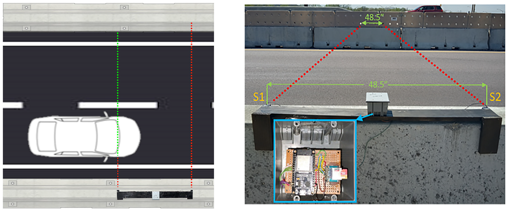
Schematic diagram and picture of the data collection device in a work zone.
Study Locations
The research team used the following criteria to identify work zones for this study: two open lanes, concrete barrier on either side, and shy distance to barrier of 1 or 2 ft. Data were collected at 17 locations across Illinois, Michigan, and Wisconsin. The attributes of these locations are shown in Table 1. All the locations had two open lanes in the work zone. The number of lanes outside the work zone varied from two to four. All but three locations had counter-directional flow (with the traffic crossed over to the opposing side) separated by concrete barriers with glare screens. All the locations had concrete barriers on both sides with shy distances to the barrier ranging from 1 to 3 ft. The data collection device was mounted on the right-hand concrete barrier, as shown in Figure 1, for nearly two days. During the data collection, video data was recorded for up to 1 h at each location. Information about the speed limit, enforcement or speed management strategies, and any other factors that could affect speed or lane position were noted. The actual shy distance to the right-hand barrier from the edge of the pavement marking was measured in the field. The device could only be mounted on the shoulder because the traffic was counter-directional, or the median side could not be safely accessed by the research team. The Mauston work zone (locations WI-2, WI-3, and WI-4) used speed feedback signs on the approach to the work zone in both directions. None of the work zones had speed enforcement. All the locations with 1-ft shy distance were very short sections (a few hundred feet), which could affect the findings.
Attributes of Work Zone Data Collection Locations
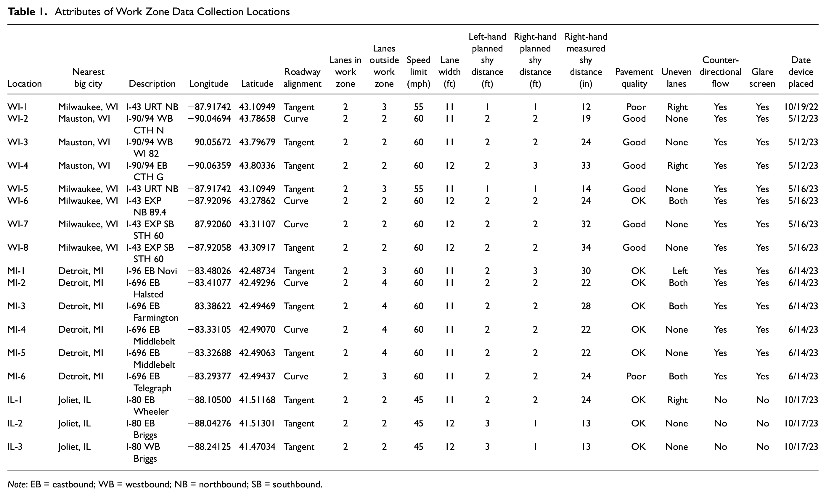
Note: EB = eastbound; WB = westbound; NB = northbound; SB = southbound.
Safety Analysis
Safety data collection and modeling have been a challenge in the context of work zones. Crashes are rare events, thankfully, and therefore do not provide robust results in situations such as work zones using a crash history approach. Simulator-based approaches are hard to validate and even the large-scale SHRP2 NDS study provided only several hundred traversals through work zones ( 16 ). Alternatively, traffic conflicts (e.g., number of encroachment events) could be considered since conflicts are more frequently observed than crashes. An encroachment-based approach has been commonly applied to develop relationships between roadside crashes and roadside conditions ( 17 , 18 ). Encroachment data, however, are not readily available, either. Tire track skid marks are often used when direct encroachment observations are not available. Given the challenges of collecting encroachment data, vehicles’ lateral position in a travel lane could serve as a surrogate safety measure and is critical to understanding the safety impact of lane width and shy distance. Therefore, the research team used the data collection device to collect large-scale lateral distance data at several work zones. This section describes the data processing, exploratory data analysis of lateral distance data, analysis and modeling methodology, modeling of lateral distance data, and finally estimating the probabilities of edge line encroachment and barrier contact.
Data Processing
The research team collected lateral distance from the right-hand side only because of the constraints mentioned in Study Locations. Consequently, the safety analysis is limited to lane departures in the right-hand lane (Lane 1). Lateral distance (from the right-hand side of the vehicle) was used as a surrogate safety measure to evaluate the probability of edge line encroachment or barrier contact within the work zone. For every vehicle the mean and standard deviation of the lateral distance measured at the two sensors were computed. Records with large standard deviations of lateral distance (standard deviation >80 cm or 31.5 in.) were considered as outliers and excluded from the data analysis. The subsequent analysis utilized lateral distance data from right-hand lane vehicles with reliable speed information, totaling 273,269 vehicles across all 17 locations.
Sunrise and sunset times for the specific days of data collection were used to assign day, night, dawn, and dusk to each observation. Observations from sunset to 1 h after were assigned dusk and observation from 1 h before sunrise to sunrise were assigned dawn. The observations between sunrise and sunset were assigned day and the rest were assigned night. Dawn and dusk observations were not included in the comparison between day and night conditions.
Exploratory Data Analysis
Table 2 presents summary statistics of lateral distance to the edge line according to lane width and shy distance. For each location, the speed limit, lane width, planned shy distance to the barrier, and actual shy distance measured at the time of data collection are presented. For lateral distance, the count of vehicles, minimum, maximum, average, standard deviation, and average during day and night are shown. The vehicle count ranged from 2000 to over 35,000. Overall, data from more than a quarter million vehicles was used for the safety analysis and modeling.
Summary Statistics of Lateral Distance to Edge Line by Lane Width and Shy Distance
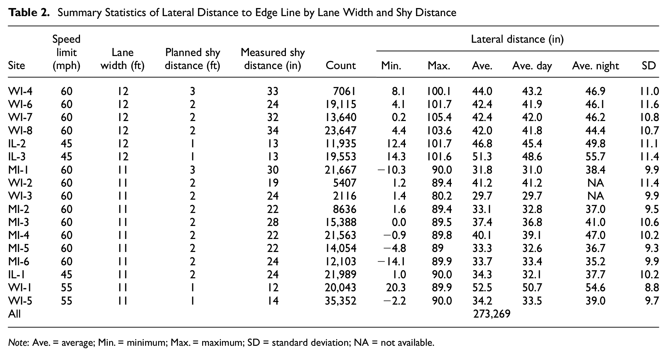
Note: Ave. = average; Min. = minimum; Max. = maximum; SD = standard deviation; NA = not available.
Readers should note that the actual shy distance to the barrier could differ from the planned shy distance. The actual shy distance was used to compute the distance to the edge line and distance to the barrier. As one might expect, the average lateral distance to the edge line varies between different locations. Interestingly, the average lateral distance to the edge line increases during the night compared with daytime at all the locations. The differences in the averages range from 1.8 to 7.9 in. This finding is intuitive as drivers tend to veer away from the edge line at night because of visibility constraints. At two of the Mauston locations (WI-2 and WI-3), the right-hand lane was closed during the night. Therefore, the average lateral distance to the edge line at night is not available for these two locations.
The probability density functions (PDFs) for lateral distance to the edge line at each location are depicted in Figure 2. The PDFs of locations with identical lane width and shy distance are shown in the same color. One can notice the variability within the same-colored plots is less than the variability with the other-colored plots. One exception is the group with locations WI-1 and WI-5. These are both at the same location: I-43 NB URT under the Overleaf trail. The difference was WI-1 was on older poor-quality pavement that used the shoulder for the right-hand lane, while WI-5 was on the crossed-over, reconstructed/new pavement. The team surmises that the significant difference between these two locations can be attributed to this reason.
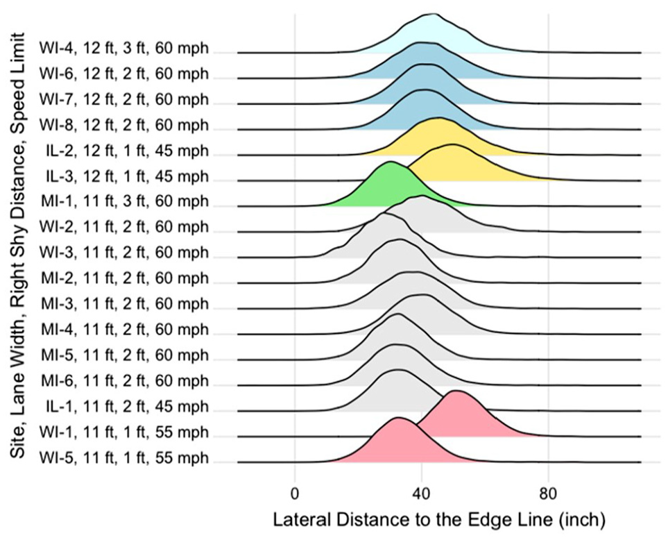
Empirical probability density function of lateral distance to the edge line.
For a given lane width, as the shoulder width or shy distance to the barrier increases, one can expect drivers to move closer to the edge line. In other words, the lateral distance to the edge line decreases, and this trend is confirmed in Figure 2. Readers should note that the amount of decrease in lateral distance to the edge line is smaller than the increase in the shy distance. In other words, while drivers move closer to the edge line, they are farther from the barrier because of the increase in the shy distance. For a given shy distance to the barrier, as lane width increases, the lateral distance to the edge line increases. This trend can also be observed in Figure 2. The PDFs for lateral distance to the right-hand barrier were examined and show that the lateral distance to the barrier increases as the lane width or the shy distance to the barrier increases, as one would expect.
The exploratory data analysis provides the following intuitive findings:
lateral distance to the edge line increases during nighttime compared with daytime;
lateral distance to the edge line increases with wider lanes and decreases with wider shy distances;
lateral distance to the barrier increases with wider lanes and wider shy distances.
Analysis and Modeling Methodology
The safety analysis and modeling methodology comprised three components, as shown in Figure 3. Firstly, all the observations, represented by the average lateral distance to the edge line/barrier, were modeled. Next, tail events, represented by the lowest one percentile of the lateral distance observations, were modeled. Finally, the probabilities of edge line encroachment and barrier contact were modeled. All events and tail events were modeled using the standard linear regression approach. The methodology used to model the probabilities of edge line encroachment and barrier contact is described next.
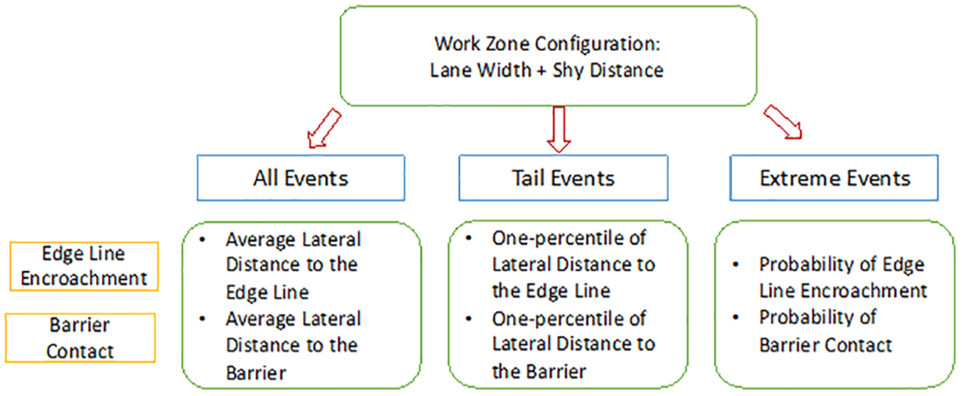
Overview of safety analysis.
EVT is used to estimate the likelihood of edge line encroachment and contact with the right-hand side barrier. EVT estimates crash risk by analyzing all traffic events, bypassing the need for crash data. In this study, the peak over threshold (POT) method with a generalized Pareto (GP) distribution is used for the EVT modeling. The POT method quantifies the stochastic behavior of processes at extreme levels by considering conflicts surpassing specific thresholds. For instance, in Figure 4, surrogate safety measures surpassing severity thresholds (S2) are identified as exceedances or risky events. These exceedances are then used for EVT modeling to predict the probability of extreme events (S3).
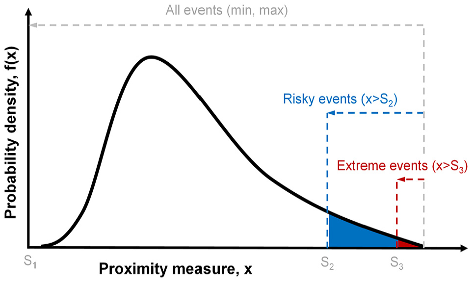
Illustration of extreme value theory modeling.
EVT focuses on the tail of the distribution, with less frequent exceedances occurring as severity increases. The GP distribution, selected for its applicability to tail events surpassing thresholds, is employed to model exceedance distributions. This GP distribution is defined as follows ( 19 ):

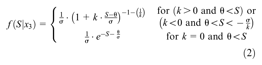
where
Using the statistical tool R, the research team applied the GP distribution with the POT method to model exceedances, providing shape and scale parameters for computing conditional probabilities of extreme events. When modeling lateral distance, the focus was on extreme values, so the negative values of lateral distance to the edge line were utilized in the POT. The optimal threshold (S2) was identified to ensure statistical reliability and model validity.
Two types of lane departure events were evaluated: edge line encroachment and barrier contact. For edge line encroachment events, where lateral distance is less than zero, S3 was set to 0. For barrier contact events, where lateral distance is less than the negative of shy distance, S3 was set to the negative of shy distance. The conditional probability of extreme events given risky events was estimated using the GP distribution. The probability of extreme events was calculated by multiplying the estimated conditional probability by the empirical probability of risky events (the number of exceedances over the number of total observations).
Modeling of All Events and Tail Events
All Events
The average lateral distances to the edge line and average lateral distances to the barrier represent all events and are shown in Figure 5, a and b , respectively. The plots illustrate that vehicles on wider lanes tend to move farther from the edge line and barrier. Conversely, with greater right-hand shy distance to the barrier, vehicles tend to move closer to the edge line but farther from the barrier. Linear regression models were developed to generalize the findings and are presented in Table 3. In these models, lateral distances to the edge line and barrier served as the dependent variables, while lane width and shy distance were independent variables. Both models demonstrate good performance, with lane width and shy distance showing statistical significance (p-value < 0.01). Figure 5, a and b , also illustrates the effects of lane width and shy distance using the estimates from the regression models.
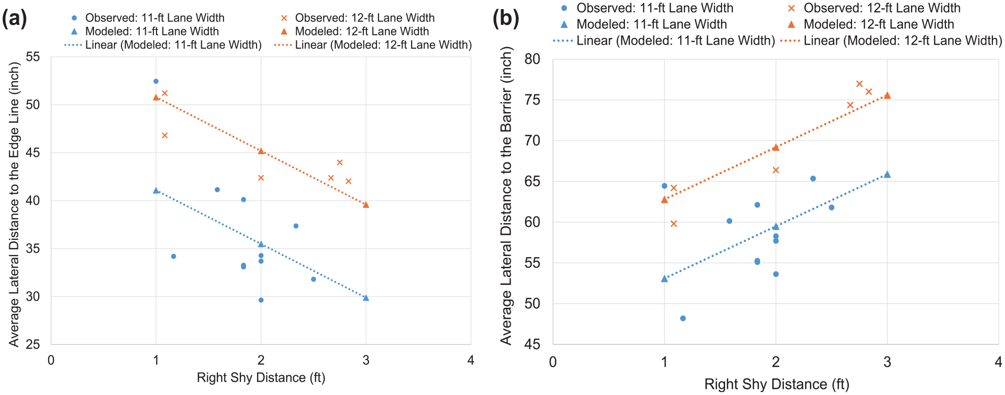
Observed and modeled average lateral distances. (a) Observed and modeled average lateral distance to the edge line. (b) Observed and modeled average lateral distance to the barrier.
Regression Analysis of Average Lane Position
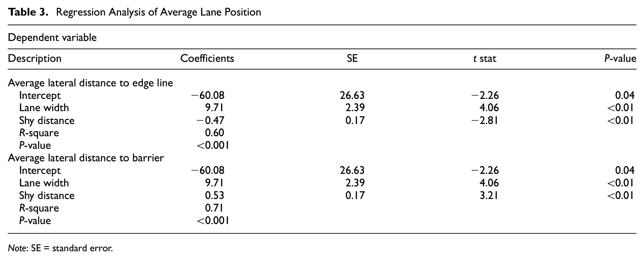
Note: SE = standard error.
Vehicles on wider lanes (12 ft compared to 11 ft) tend to stay farther away from the edge line and the barrier. Interestingly, with an additional 1-ft shy distance, vehicles move about 6 in. closer to the edge line and an additional 6 in. farther from the barrier. Therefore, with greater right-hand shy distance to the barrier, vehicles tend to move closer to the edge line but farther from the barrier.
Tail Events
Tail events are represented by the lowest one percentile of the lateral distance observations. Tail events are similar to risky events, shown in Figure 4, which have a high chance of becoming extreme events (edge line encroachment or barrier contact). The one-percentile lateral distance to the edge line and one-percentile lateral distance to the barrier for different work zone configurations are plotted in Figure 6. The plots indicate that the one percentile of vehicles on wider lanes tends to move farther from the edge line and the barrier. The one percentile of vehicles on wider shoulders tends to move closer to the edge line but farther from the barrier. These observations were corroborated using linear regression models, as depicted in Table 4. Both models demonstrate good performance, with lane width and shy distance showing statistical significance (p-value < 0.01). The patterns of lateral distances to the edge line and barrier are similar to the patterns observed with average lateral distances.
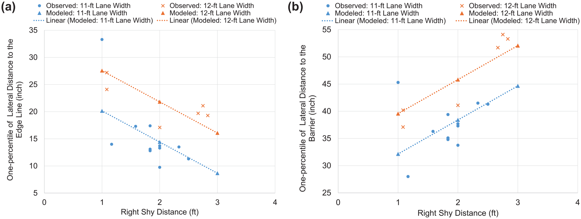
Observed and modeled one-percentile lateral distances. (a) Observed and modeled one-percentile lateral distance to the edge line. (b) Observed and modeled one-percentile lateral distance to the barrier.
Regression Analysis of Tail Lane Position
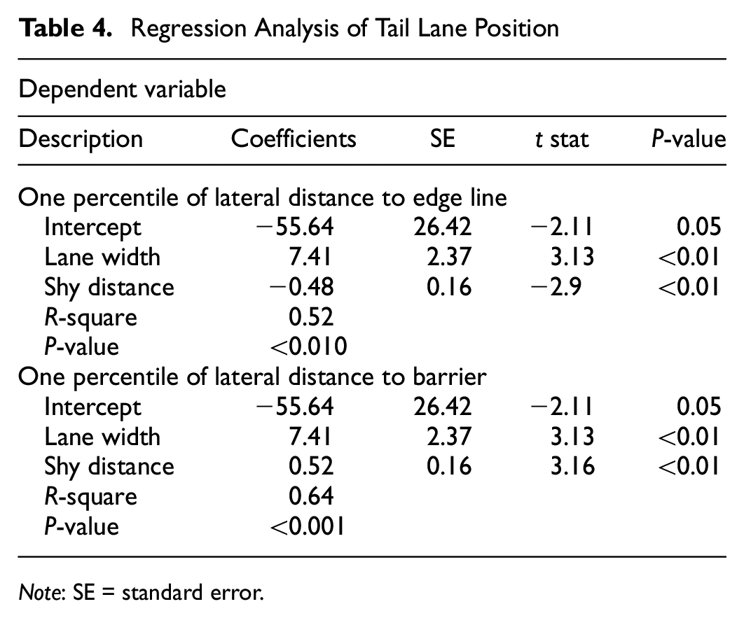
Note: SE = standard error.
Probability of Edge Line Encroachment and Barrier Contact
The research team developed a comprehensive EVT model utilizing data from all the sites to capture the impact of all the variables of interest. This approach provided more exceedances when compared to developing EVT models for individual locations. The full model is non-stationary and incorporates covariates in the scale parameter estimation. The shape parameter remains unchanged because of the absence of factual evidence indicating non-stationarity in tail behavior; thus, no covariates were included in its estimation ( 19 ).
The covariates considered are lane width, shy distance, road curvature, and speed limit, along with vehicle-level variables including time of day (day or night), free flow conditions, vehicle type (passenger car or truck), and adjacency to other vehicles. Various combinations of these variables were assessed using the likelihood ratio test to streamline model structures and variable inclusions. The non-stationary model, which incorporates a linear combination of lane width and shy distance in the scale parameter, exhibits significance with a small p-value of 0.02 in a likelihood ratio test compared with the stationary model. However, when additional terms or interaction terms are included in the linear combination, the model loses significance.
Consequently, the final model incorporates a linear combination of lane width and shy distance in the scale parameter. The optimal threshold of 12 in. resulted in 1147 exceedances that were used to develop the EVT model. As depicted in Table 5, a negative scale parameter for lane width signifies that an increase in lane width reduces the scale parameter and, consequently, the variance of the lateral distance distribution and a decrease in the probability of extreme events. Conversely, a positive scale parameter for shy distance indicates that an increase in shy distance augments the scale parameter and the probability of extreme events. The shape parameter is not statistically significant, but it is retained in the final model because it provides a better fit compared to the model with a zero-value shape parameter.
Estimation Results for the Extreme Value Theory Model
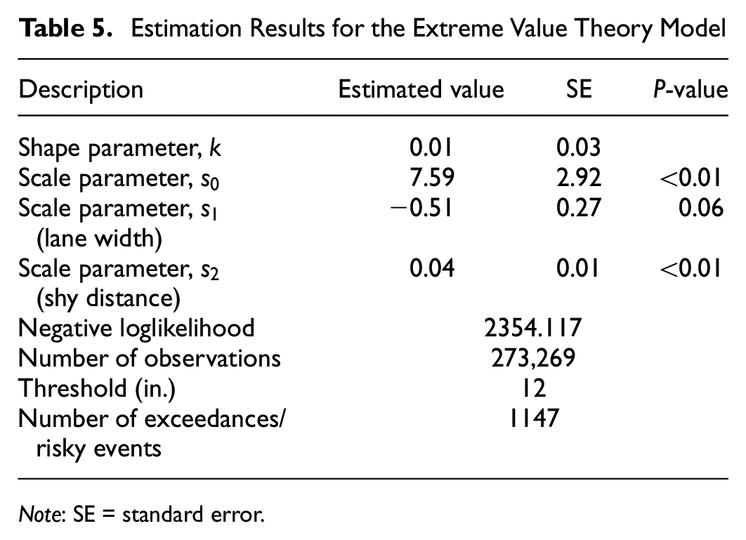
Note: SE = standard error.
Figure 7 illustrates the impact of lane width and shy distance on the probability of edge line encroachment and barrier contact. An increase in lane width leads to a reduction in the probability of edge line encroachment and barrier contact. An increase in shy distance results in an increase in the probability of edge line encroachment and a decrease in the probability of barrier contact. For an 11-ft lane, the probability of barrier contact approaches zero for a 3-ft right-hand shy distance. Similarly, for a 12-ft lane, the probability of barrier contact approaches zero for a 2-ft shy distance.
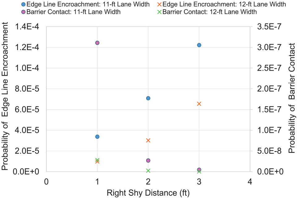
Impact of lane width and shy distance on extreme events.
Mobility Analysis
Mobility analysis focused on free flow speed, given its vital role in estimating other mobility impacts such as capacity and queue length. Researchers have used different headway thresholds to define free flow vehicles. Cantisani et al. ( 20 ) provide a detailed review of the literature on this topic. Evans and Wasielewski ( 21 ) examined headways on freeways and suggested a headway threshold of 2.5 s for traffic flow of less than 1450 vehicles per hour per lane and 3.5 s for higher flow levels. Wasielewski ( 22 ) examined a semi-Poisson headway distribution model and suggested a 4.0-s headway threshold for freeways. Susarak et al. ( 23 ) studied multilane highways and defined a headway threshold of 3.0 s for passenger cars and 4 s for heavy vehicles. Benekohal et al. ( 24 ) used a 4.0-s threshold for vehicles in work zones on freeways. One study used a 5.0-s threshold on freeways ( 25 ). Other studies on two-lane highways suggested headway thresholds ranging from 2.5 to 9.0 s for identifying free flow vehicles ( 26 – 39 ). Since the 4.0-s threshold was the most recommended/used for freeways in the literature, the same was used in this research.
The speed analysis was limited to free flow vehicles with reliable speed estimates. Standard outlier analysis was performed to remove the outliers using the interquartile range before performing any other analysis. A summary of the number of observations and speed descriptive statistics for each location is provided in Table 6. Overall, speed data from 125,447 free flow vehicles was used and the number of free flow vehicles at individual locations ranged between 2000 and 15,000. Free flow vehicles in both lanes were included in the analysis. The posted speed limits for all the three sites in Illinois were 45 mph, for two sites in Wisconsin were 55 mph, and for the rest of the sites were 60 mph. The average speed ranged between 54 and 70 mph, which was highly associated with the posted speed limit. The difference between the average speed and speed limit ranged between −0.8 and 14.1 mph, which indicated that the average speed was as high as 14.1 mph over the speed limit or 0.8 mph under the speed limit. WI-1 had 11-ft lanes with 1-ft shy distance, poor pavement, with the old shoulder as the right-hand lane, and was immediately upstream of an exit ramp. These factors probably contributed to the free flow speed being lower than the speed limit.
Summary of Speed Data
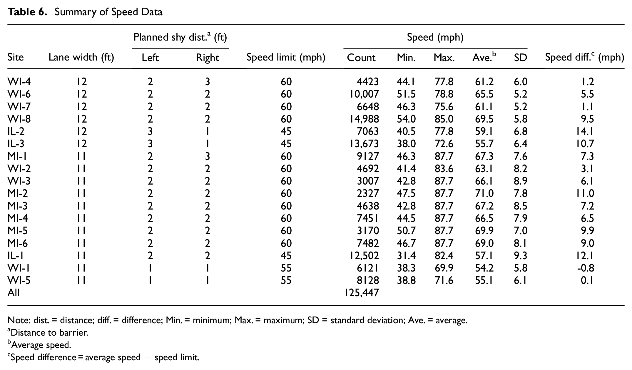
Note: dist. = distance; diff. = difference; Min. = minimum; Max. = maximum; SD = standard deviation; Ave. = average.
Distance to barrier.
Average speed.
Speed difference = average speed − speed limit.
The PDFs for free flow speed at each location are depicted in Figure 8. The PDFs of locations with identical lane width and shy distance are shown in the same color. One can note that, in general, the variability within the same-colored plots is less than the variability with other-colored plots. The one exception is the group with locations WI-6, WI-7, and WI-8. WI-7 has lower free flow speeds than the other two locations although they share the same geometry. WI-7 was about a quarter mile downstream of an entrance ramp and that could have contributed to the lower free flow speeds at this location.
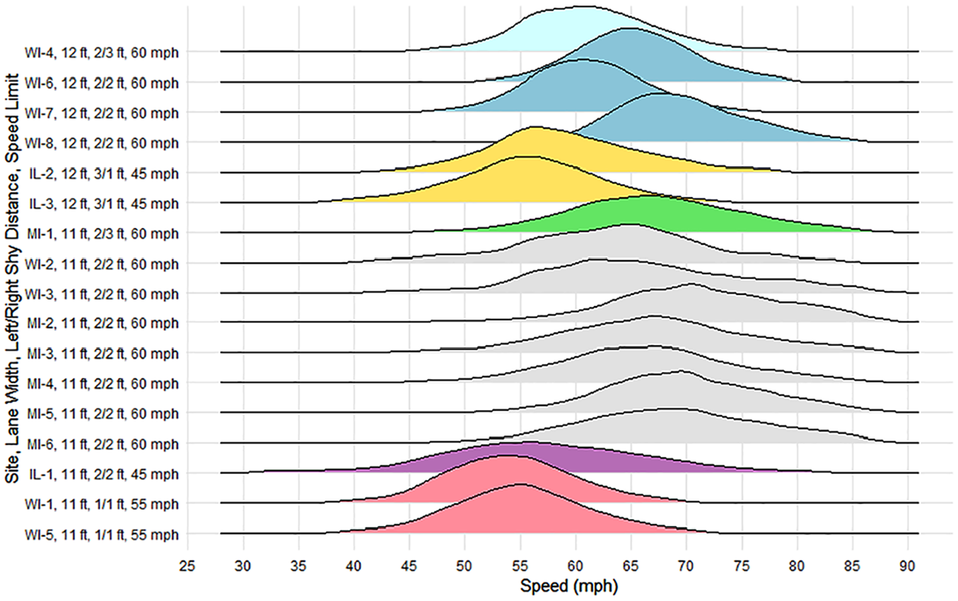
Empirical probability density function of free flow speed by location.
Analysis and Modeling Methodology
Linear regression was used in this research to model free flow speeds. The HCM uses the same approach to relate free flow speed to variables of interest ( 6 ). Linear regression is a statistical modeling approach that establishes linear relationships between the response and exploratory variables. The least squares approach was implemented to fit the model to the observed data. The method consists of minimizing the sum of the squares of vertical deviations in each data point. Model coefficients contribute to evaluate the effects of predictor variables. Linear regression has the following model form:
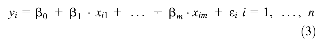
A correlation analysis was implemented to evaluate the statistical relationship of variables considered for modeling speed. Through regression modeling, linear regression models were developed with speed as the dependent variables and geometric and operational measures as the independent variables. Measures of goodness of fit include the statistical significance of model coefficients, confidence intervals, and R-square.
Free Flow Speed Estimation
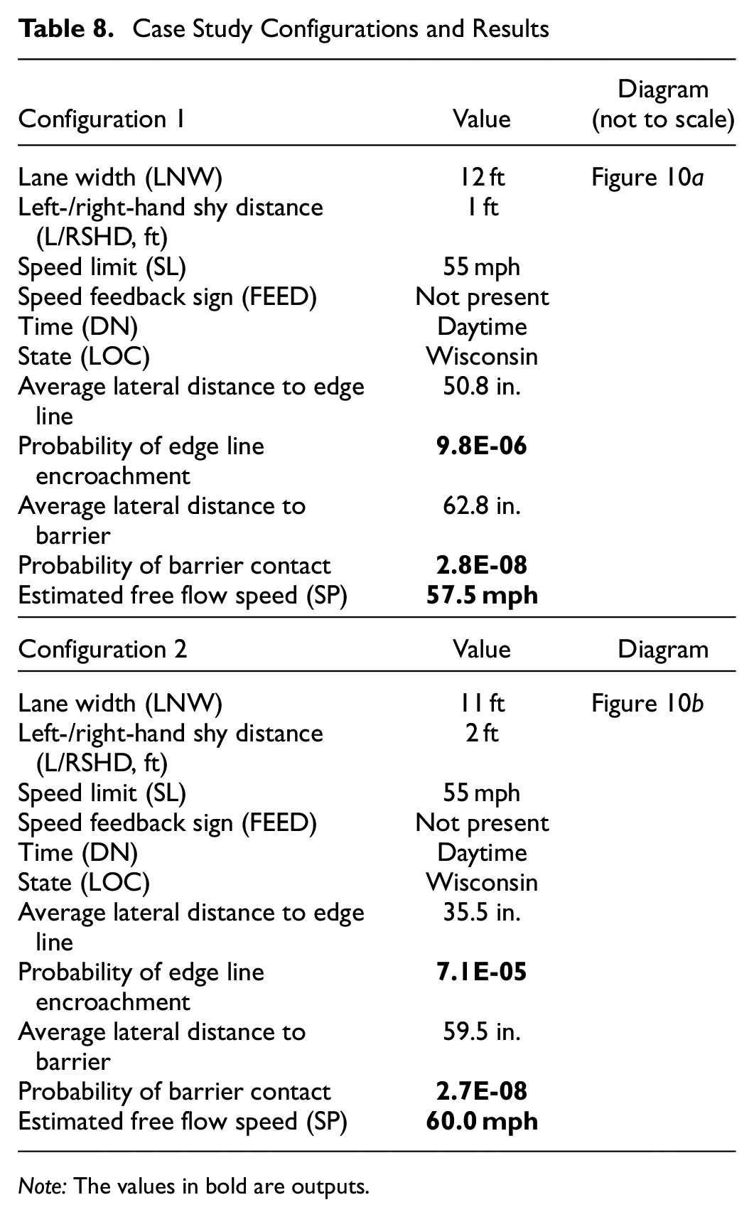
Using speed data, linear regression was implemented to develop models to predict free flow speeds at work zones with geometric and operational variables. In preparation for modeling, data distribution and availability were reviewed for every predictor variable. Five locations had a smaller number of reliable speed observations in the left-hand lane. Data from the left-hand lane were only available for 2%–17% of the overall observations at those locations. Thus, the decision was made to exclude those locations for modeling since there would have been an overrepresentation of observations from right-hand lane, which could have introduced a bias in the model estimates. As a result, the 12 locations that had at least 25% of observations in the left-hand lane were included in the model. A total of 94,200 observations were used for the regression modeling. A model was developed by work zone, so designers can estimate free flow speed in work zones at the design stage based on the speed limit, geometry, day/night, and presence of speed feedback signs. The model is provided in Equation 4 and, as one would expect, free flow speeds increase with an increase in lane width, shy distance, and speed limit. The results also show that work zone free flow speeds are statistically significantly higher under nighttime conditions when compared to daytime conditions, which differs from the HCM ( 6 ). The model suggests that free flow speeds increase in order from Wisconsin, Michigan, and Illinois. This could very well be because of the differing speed limit policies of the different states. The speed limit was the lowest in Illinois work zones at 45 mph; followed by Wisconsin, which had two locations with 55 mph speed limits and 60 mph in the rest; while all the locations in Michigan had 60 mph speed limits. Table 7 includes the model coefficients and measures of goodness of fit:
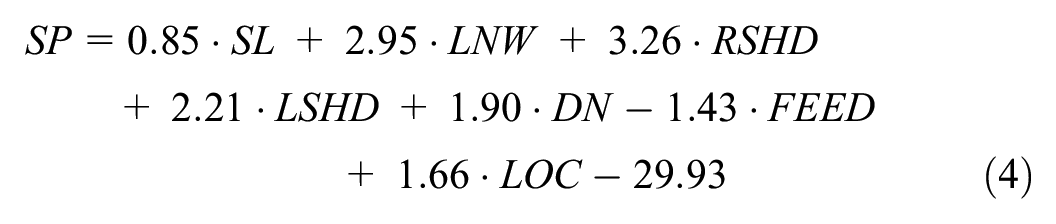
where
Regression Model Coefficients and Goodness of Fit Measures
Note: SL = posted speed limit (mph); LNW = lane width (ft); RSHD = right shy distance to barrier (ft); LSHD = left side distance to barrier (ft); DN = time of the day (day or night); FEED = speed feedback sign (not present or present); LOC = site location (WI, MI, IL); SE = standard error.
As one would expect, free flow speeds increase with an increase in lane width, shy distance, and speed limit. The results also show that work zone free flow speeds are higher under nighttime conditions when compared to daytime conditions. The higher speeds at night observed in our data and found statistically significant in the linear regression differ from the HCM’s finding in this regard ( 6 ). The model suggests that free flow speeds increase in order from Wisconsin, Michigan, and Illinois. This could very well be because of the differing speed limit policies of the different states. The speed limit was the lowest in Illinois work zones at 45 mph; followed by Wisconsin, which had two locations with 55 mph speed limits and 60 mph in the rest; while all the locations in Michigan had 60 mph speed limits.
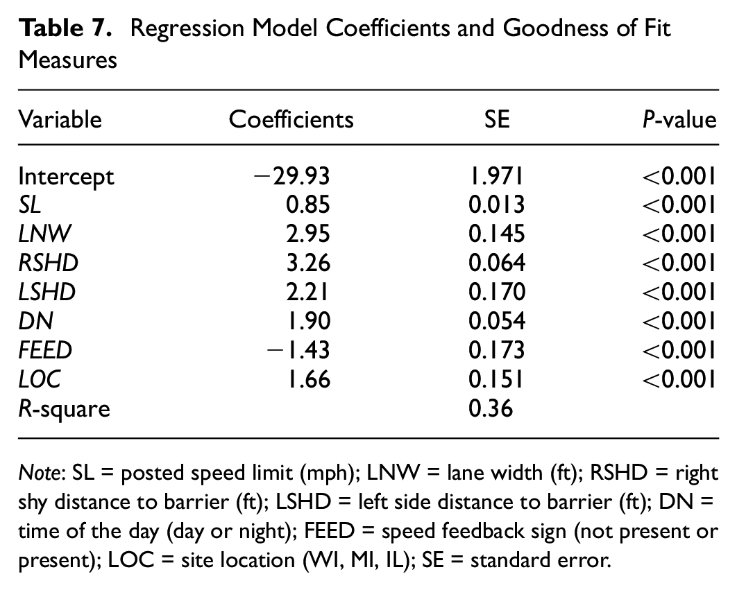
Figure 9 was developed to illustrate the impact of geometric and operational variables such as lane width (LNW), left- and right-hand shy distances (LSHD and RSHD), speed limit (SL), daytime conditions, speed feedback sign not present, and considering Wisconsin drivers.
Predicted free flow speed for Wisconsin work zones.
Case Study
The objective of this research and analyses was to enable a comparison between multiple lane width and shy distance configurations for a given paved width. This section presents a case study of 26-ft available paved width for a 55-mph posted work zone with two open lanes, with a barrier on both sides. The two geometric configurations are as follows:
lane widths of 12 ft with left- and right-hand shy distances of 1 ft; and
lane widths of 11 ft with left- and right-hand shy distances of 2 ft.
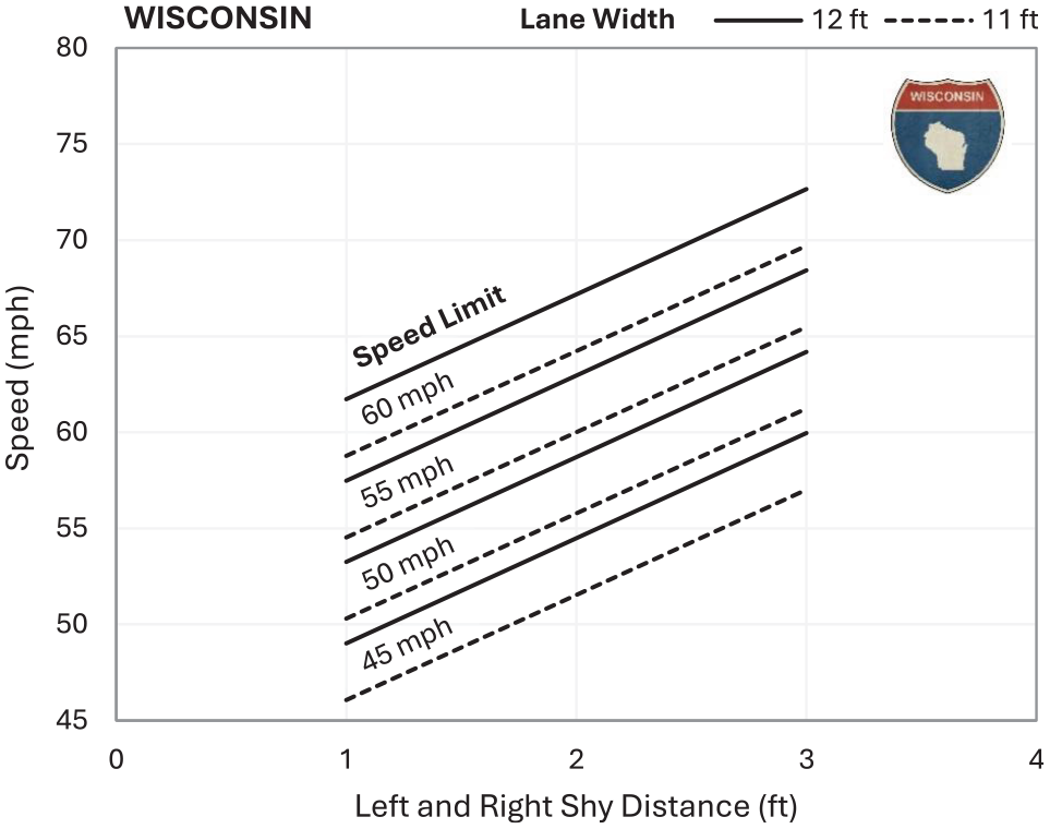
For speed modeling in this case study, the work zone is assumed to be in Wisconsin, conditions are daytime, and no speed feedback sign is present. The estimated probabilities of edge line encroachment and barrier contact are not affected by day/night. Data and results for the two geometric configurations are provided in Table 8.
Case Study Configurations and Results
Note: The values in bold are outputs.
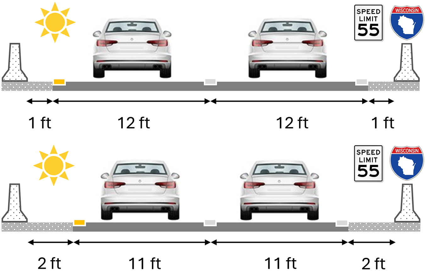
Geometric configurations for case study
Under Configuration 1 (12-ft lanes, 1-ft shy distances), on average, vehicles in the right-hand lane are expected to be 50.8 in. from the right-hand edge line and 62.8 in. from the right-hand barrier. Under Configuration 2 (11-ft lanes, 2-ft shy distances), on average, vehicles in the right-hand lane are expected to be 35.5 in. from the right-hand edge line and 59.5 in. from the right-hand barrier. The average lateral distance from the edge line is much greater with the 1-ft shy distance (50.8 in.) than the 2-ft shy distance (35.5 in.). However, the average lateral distances to the right-hand barrier differ by only about 3 in.: 62.8 and 59.5 in. under Configurations 1 and 2, respectively. This suggests that the narrow shy distance greatly affects the lateral distance of vehicles, which shy away from the edge line (and barrier).
The probabilities of edge line encroachment under Configurations 1 and 2 are 9.8E-06 and 7.1 E-05, respectively. In other words, edge line encroachment is about seven times more likely with a 2-ft shy distance than a 1-ft shy distance. While this may appear counterintuitive, this trend is to be expected. Drivers position their vehicles with respect to the barrier. Under narrower shy distances drivers tend to shy away from the barrier and therefore it is less likely that they will encroach beyond the edge line. From a safety perspective, the real concern is vehicles making contact with the barriers. The probabilities of barrier contact under Configurations 1 and 2 are 2.8 E-08 and 2.7 E-08, respectively, indicating a slightly lower value for Configuration 2. While drivers may veer into the shoulder more with a 2-ft shy distance when compared with a 1-ft shy distance, the likelihood of contacting the barrier is slightly smaller for a 2-ft shy distance. This illustrates that the EVT approach is able to capture and model the interaction between lane width and shy distance.
The estimated free flow speeds are 57.5 and 60.0 mph, respectively, for Configurations 1 and 2. In both cases, the free flow speed would be higher than the set speed limit. As stated earlier, for estimating free flow speed, the work zone is assumed to be in Wisconsin, daytime conditions, and absence of speed feedback signs. Free flow speeds would be higher by 3.3 mph in Illinois and 1.7 mph in Michigan, 1.9 mph higher during the night, and 1.4 mph lower with a speed feedback sign.
The results from this case study indicate that Configuration 2 (11-ft lanes, 2-ft shy distances) has a slightly lower probability of barrier contact than Configuration 1 (12-ft lanes, 1-ft shy distances) while having a greater free flow speed. These findings suggest that 11-ft lanes with a 2-ft shy distance is better than 12-ft lanes with a 1-ft shy distance from safety as well as mobility perspectives. While there are limitations for the safety and mobility modeling in this research effort, this finding concurs with existing guidance in the AASHTO Green Book, the Roadside Design Guide, and the work zone design guidance of multiple states.
Conclusions, Limitations, and Recommendations
The goal of this project was to quantify the mobility and safety impacts of different combinations of lane width and shy distance to the barrier for a given paved width. Data from 17 work zone locations across Illinois, Michigan, and Wisconsin were used for the analysis. All 17 locations were in long-term work zones and had two lanes open in the work zone with a concrete barrier on either side. The lane widths were either 11- or 12-ft and the left-/right-hand shy distances to barrier were 1-, 2-, or 3-ft.
Vehicle lateral position in the right-hand travel lane was used as a surrogate safety measure to understand the safety impact of lane width and shy distance. Lateral distance data of over a quarter million vehicles were used for the safety analysis. The safety analysis only considered right-hand departures for vehicles in the right-hand lane. Lateral distances indicated that, compared to the daytime, vehicles moved away from the edge line and barrier in the nighttime. Modeling of all vehicles and tail vehicles (one percentile of lateral distance) was accomplished by linear regression. Vehicles tend to move farther from the edge line and the barrier on 12-ft lanes when compared to 11-ft lanes. Vehicles tend to gravitate closer to the edge line but farther from the barrier with larger shy distances (3 ft compared to 2 and 1 ft). EVT modeling was conducted to estimate the probabilities of right-hand edge line encroachment and right-hand barrier contact. Wider lanes were found to contribute to decreased probabilities of edge line encroachment and barrier contact, while wider shy distances were associated with increased probability of edge line encroachment and decreased probability of barrier contact.
Free flow vehicle speeds of over 125,000 vehicles were used to understand the mobility impact of lane width and shy distance. Unlike the safety analysis, which only considered vehicles in the right-hand lane, mobility analysis considered vehicles in both lanes. Linear regression modeling was conducted to develop a model for estimating free flow speeds in work zones based on geometric and operational variables. The model trends with respect to the impact of the various variables are as expected: work zone free flow speed increases with an increase in speed limit, lane width, and left-/right-hand shy distance to the barrier. Nighttime free flow speeds were higher than daytime and speed feedback signs reduced the free flow speeds. Compared to Wisconsin, speeds were higher in Michigan and even higher in Illinois.
A case study of a 55-mph posted work zone speed limit with two open lanes in each direction and barrier on both sides is presented. Safety and mobility impacts of two geometric configurations, (1) lane widths of 12 ft with left- and right-hand shy distance of 1 ft and (2) lane widths of 11 ft with left- and right-hand shy distance of 2 ft, are evaluated. The results indicate that Configuration 2 has a slightly lower probability of right-hand barrier contact (for vehicles in the right-hand lane) than Configuration 1, while having a greater free flow speed. These findings suggest that 11-ft lanes with a 2-ft shy distance are better than 12-ft lanes with a 1-ft shy distance from safety as well as mobility perspectives.
As with all research, these findings are subject to limitations. The safety analysis only considered right-hand departures of vehicles in the right-hand lane. Only four locations had a 1-ft shy distance and were all very short sections (a few hundred feet). A more uniform distribution of speed limits across the different states would have been preferred. Only one location had a speed feedback sign. However, this research has demonstrated how lateral distance and speed data can be modeled. Future research efforts should embark on a larger data collection effort to capture greater variability in the different parameters and obtain lateral distance from both sides to estimate lane departures in both directions and for vehicles in both lanes. Future research could consider the impact of weather or pavement condition.
Footnotes
Author Contributions
The authors confirm contribution to the paper as follows: study conception and design: M.V. Chitturi, G. Vorhes, data collection: M.V. Chitturi, G. Vorhes, analysis and interpretation of results: M.V. Chitturi, G. Vorhes, Z. He, B. Claros, manuscript preparation: M.V. Chitturi, G. Vorhes, Z. He, B. Claros, X. Qin, A.R. Bill, D.A. Noyce. All authors reviewed the results and approved the final version of the manuscript.
Declaration of Conflicting Interests
The author(s) declared the following potential conflicts of interest with respect to the research, authorship, and/or publication of this article: X. Qin is a member of Transportation Research Record’s Editorial Board. All other authors declared no potential conflicts of interest with respect to the research, authorship, and/or publication of this article.
Funding
The author(s) disclosed receipt of the following financial support for the research, authorship, and/or publication of this article: This research was supported by the Smart Work Zone Deployment Initiative (SWZDI) and Federal Highway Administration (FHWA) Pooled Fund Study TPF-5(438).
ORCID iDs
Data Accessibility Statement
Data will be made available on request.