






Abstract
Sidewalk condition plays a critical role in ensuring pedestrian safety, accessibility, and compliance with regulatory standards. Conventional assessment methods typically involve manual inspections using categorical ratings, which are labor-intensive, subjective, and limited in spatial coverage. This study evaluates the use of satellite imagery and machine learning to support sidewalk condition assessments. A classification model was developed using synthetic aperture radar (SAR) imagery combined with sidewalk physical attributes, including width, slope, and material type. A random forest classifier was trained to predict four condition categories: good, fair, poor, and severe. To address the substantial imbalance in the distribution of classes, a binary formulation was also tested by grouping segments into defective and nondefective classes. Data resampling techniques combining under- and oversampling were applied to improve model performance. The results indicated that the binary model with combined sampling achieved the best performance, with a recall of 0.85 and G-mean of 0.81. Models trained on the original four classes showed lower performance owing to underrepresentation of the poor and severe categories. Feature-importance analysis highlighted SAR amplitude as the most influential predictor across all scenarios. The findings demonstrated the potential of SAR imagery to support scalable and data-driven evaluation of sidewalk conditions. This approach offers a viable complement to traditional inspection methods by enabling targeted resource allocation and broader spatial coverage in pedestrian infrastructure management.
Keywords
Introduction
Maintaining safe and accessible sidewalks is critical for transportation agencies. Sidewalks in good condition enable pedestrian safety and mobility, especially for people with disabilities, seniors, and others who rely on barrier-free paths ( 1 ). Regular sidewalk inspections are essential to identify hazards (e.g., cracks, heaves, and obstructions). Federal guidance emphasizes that proactive inspections can help reduce slips and falls and ensure accessibility, noting that damaged or uneven sidewalks can become impassable and limit access for individuals with disabilities ( 2 ). Ensuring compliance with the Americans with Disabilities Act (ADA) is also a key motivator; sidewalk segments that do not meet ADA standards are often unsafe, exposing users (e.g., wheelchair users or those with strollers) to unnecessary risks ( 3 ). Thus, systematic inspections support not only public safety and mobility, but also legal compliance and equity in the transportation network ( 2 ).
Many agencies lack comprehensive inventories or condition datasets for sidewalk infrastructure ( 2 , 4 ). A recent study on municipal sidewalk inventories in the United States ( 5 ) found that the mean and median costs to conduct sidewalk inventories are $283 and $192/mi, respectively. Including sidewalk condition assessments within inventory efforts requires significantly more time and large inspection teams. The City of Seattle, WA, for example, spent approximately $400,000 to conduct a condition assessment of sidewalks that employed 17 interns, whereas the City of Austin, TX used 15 to 20 sidewalk crews to perform its condition assessment ( 5 ). The high costs of these inspections result in limited data available on sidewalk conditions. A recent nationwide study on ancillary assets found that less than a third of state departments of transportation (DOTs) in the United States (i.e., 10 out of 37 respondents) are currently inspecting sidewalks ( 6 ). The lack of condition data hinders the capacity of agencies to perform data-driven decisions, resulting in suboptimal management decisions.
When performed, sidewalk condition assessments rely heavily on manual field inspections ( 7 – 9 ). Crews typically walk the sidewalks and classify each segment based on visual signs of surface distress, using condition indices (e.g., the Sidewalk Condition Index [ 10 ]) or ratings. An example of this rating system, used by the Minnesota Department of Transportation (MnDOT) classifies sidewalk condition under four categories: good, fair, poor, or severe (Figure 1). However, manual inspections are labor-intensive, subject to observer variability, and offer limited spatial and temporal coverage ( 11 ). These challenges hinder data-driven decision making. This study explores a scalable alternative using satellite-based synthetic aperture radar (SAR) imagery combined with sidewalk attribute data to predict condition. The goal is to support infrastructure monitoring through automated, repeatable assessments that complement traditional field inspections.
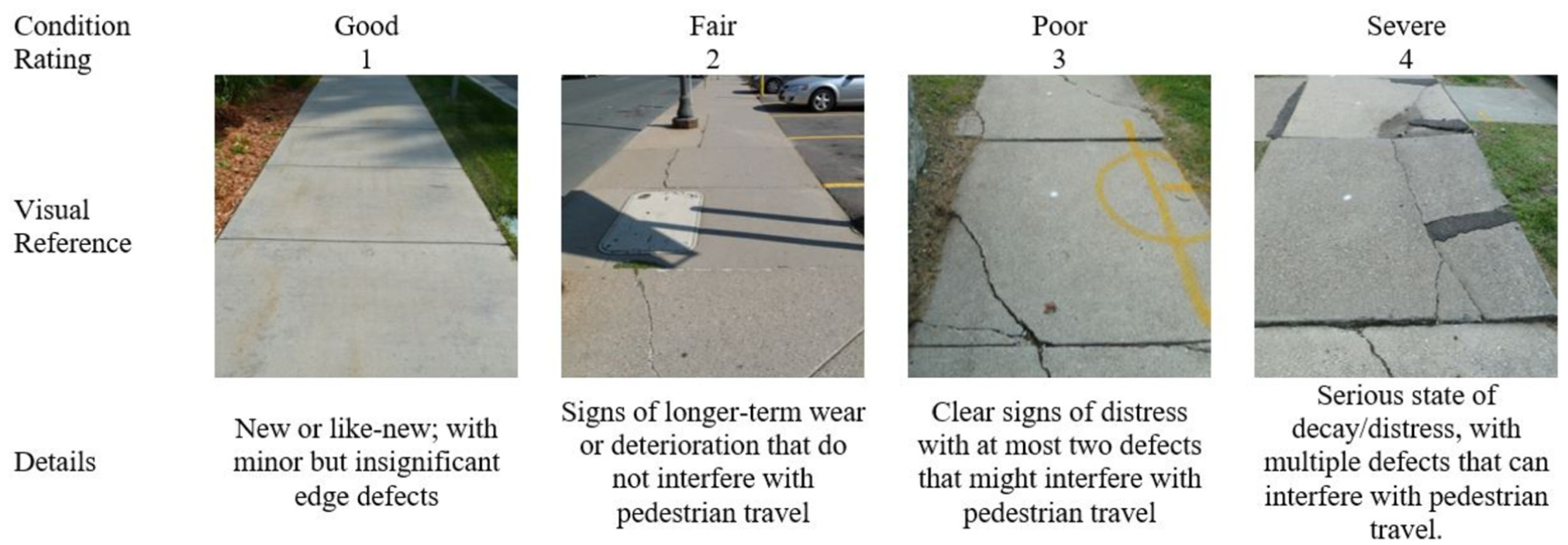
Minnesota Department of Transportation’s sidewalk condition rating scale.
Literature Review
Traditional sidewalk condition assessments are typically conducted through manual, in-person inspections, where crews visually identify surface defects such as cracks, spalling, or vegetation intrusion. These methods often rely on categorical ratings ( 8 , 9 ). Although widely used, manual inspections face several limitations. First, collecting condition data at scale is time- and resource-intensive; in some cases, updates occur only every few years owing to staffing or budget constraints. For example, the City of Middleton and the Village of Shorewood in Wisconsin, United States, estimate that it will take approximately 8 years to assess sidewalks across all neighborhoods ( 12 , 13 ). Second, visual assessments are inherently subjective because different inspectors may rate similar segments inconsistently without standardized benchmarks ( 14 , 15 ). Third, although many state DOTs maintain an inventory of “pedestrian assets” (e.g., ramps, signals), less than half (i.e., 45%) actually assign condition ratings to them ( 7 ). A national survey of state DOTs revealed that only 16% (6 out of 37) classify sidewalks as “condition-rated,” whereas 73% explicitly reported that they do not track condition data for these assets ( 6 ). This widespread lack of systematic condition data underscores the urgent need for scalable, remote-sensing solutions.
To address these issues, recent studies have explored the use of advanced sensing and data-driven techniques to evaluate sidewalk conditions. Mobile LiDAR systems, for example, can map sidewalk geometry with centimeter accuracy and have been used to evaluate cross-slope, width, and trip hazards relevant to ADA compliance ( 16 – 18 ). Image-based methods using cameras or drones, combined with deep learning models, have demonstrated potential for detecting cracks and other surface-level damage present in sidewalks ( 19 ). Accelerometer-based roughness detection, often via smartphones or lightweight carts, has been used for crowdsourced or low-cost surveys of pedestrian comfort ( 20 , 21 ). Devices such as the Ultra Light Inertial Profiler can collect high-resolution surface profiles, but they often miss vertical displacements between sidewalk slabs because of limited coverage ( 22 ). In the European context, researchers have developed portable systems to scan sidewalks. Examples of these advances include WalkBot, a portable system designed to scan sidewalks and collect condition-related attributes at the network level ( 23 ) and a stroller-mounted sensing system for continuous sidewalk condition monitoring ( 24 ). Although these approaches reduce inspection time, they still require on-site sensor deployment, resulting in time-intensive evaluations that limit the temporal frequency and spatial coverage of sidewalk inspections.
Remote-sensing technologies offer an opportunity to further expand monitoring capabilities. SAR seems particularly valuable because it captures imagery regardless of weather or lighting conditions and has been used to detect surface changes such as cracking or deformation in road pavements ( 15 ). SAR is an active data technology in which the satellite sensor produces its own energy and records the amount of energy reflected back by the Earth’s surface. The strength of this backscatter signal is measured by its amplitude value, which depends on three characteristics of the reflecting surface: its dielectric constant, its roughness, and its structure and orientation ( 25 ). A smooth surface (Figure 2a) will act similar to a mirror and reflect all incident energy in the opposite direction. As a result, the backscattering coefficient will be low for smooth surfaces ( 26 ) as compared to surfaces with greater roughness (Figure 2, b and c ). Previous research on roadways shows that SAR amplitude can reflect changes in surface texture linked to deterioration ( 27 , 28 ). However, it is still unclear whether this signal can capture sidewalk conditions, which are narrower than roads and surrounded by buildings and other urban features.
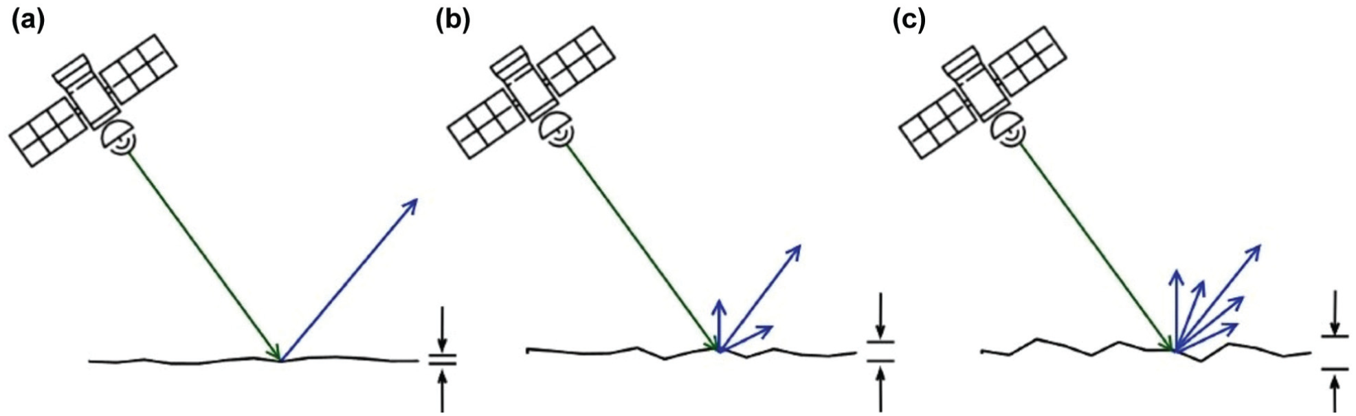
(a) Smooth surfaces will have lower SAR amplitude than (b) intermediate, and (c) rough surfaces.
Despite advances in both remote sensing for pavement monitoring and data-driven sidewalk assessment, a critical gap remains in the application of satellite-based methods to pedestrian infrastructure. Existing SAR-based studies focus on road networks, which are wider and less affected by surrounding urban features. In contrast, sidewalks are narrower, often less than 2 m in width, and are located in environments where nearby buildings and vegetation introduce mixed-pixel effects. Furthermore, sidewalk condition is typically represented using categorical ratings rather than continuous roughness indices.
This study addresses this gap by evaluating the applicability of Sentinel-1 SAR imagery for sidewalk condition classification, and by integrating satellite-derived features with sidewalk-specific attributes in a machine learning framework. This work extends SAR-based infrastructure monitoring to pedestrian networks.
The objective of this study is to develop and evaluate machine learning models that combine SAR imagery with sidewalk data to classify sidewalk condition. The goal is to enable scalable, automated, and cost-effective condition assessments that can support proactive maintenance of pedestrian infrastructure and reduce reliance on manual inspections.
Methodology
This study explores extensions of the SAR-C tool, originally developed for pavement condition assessment, to sidewalk infrastructure ( 30 ). Although SAR-C previously employed regression models for continuous pavement indicators, such as the international roughness index, the extension to sidewalks requires shifting the predictive task to a classification algorithm that reflects the categorical nature of sidewalk condition ratings (e.g., good, fair, poor, severe).
The predictive algorithm integrates two primary data sources: field-collected sidewalk condition ratings and Sentinel-1 SAR imagery. As shown in Figure 3, the process involves multiple stages, including data preprocessing, feature integration, model training, and performance evaluation.
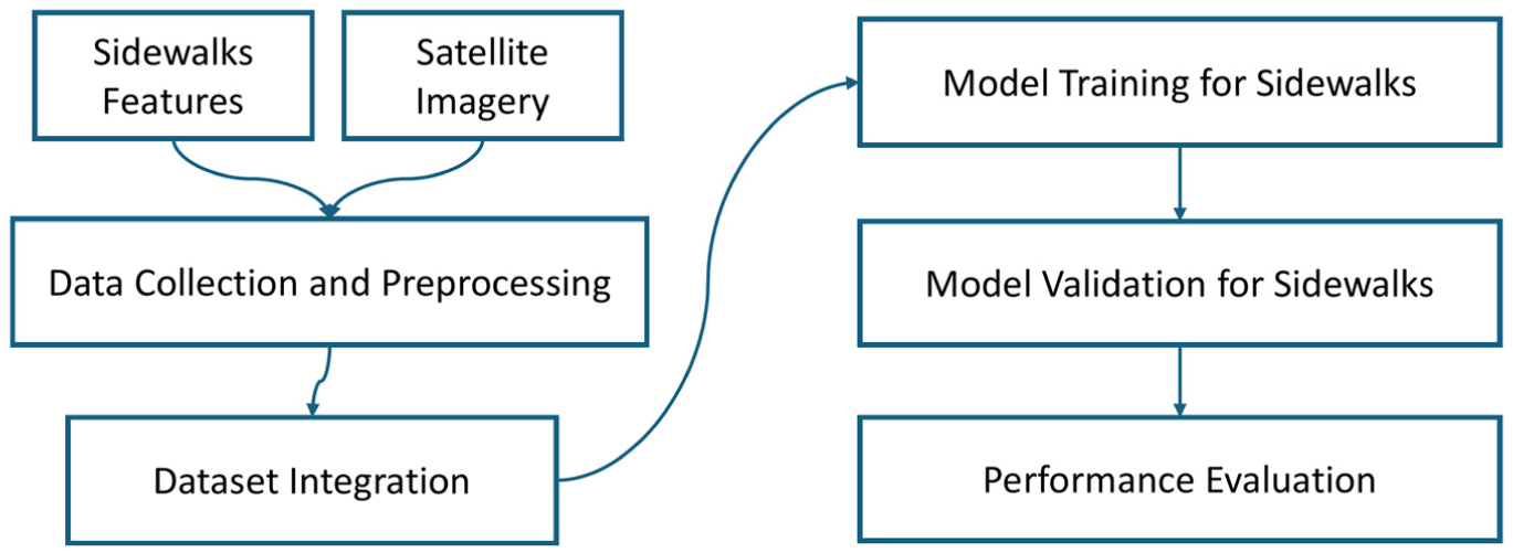
Methodology.
Data Collection and Preprocessing
Satellite Data
This study used publicly available Sentinel-1 SAR imagery from NASA’s Alaska Satellite Facility ( 31 ). Sentinel-1 is a spaceborne radar mission operated by the European Space Agency, designed to capture Earth surface data regardless of weather or lighting conditions. It uses C-band SAR with a 5.6-cm wavelength, 10-m spatial resolution, and a 12-day revisit cycle, making it well-suited for large-scale infrastructure monitoring ( 32 ). Each image covers approximately 16,700 mi2 and is defined by a unique path–frame combination. Multiple path–frame pairs were needed to achieve full coverage across Minnesota (Figure 4).
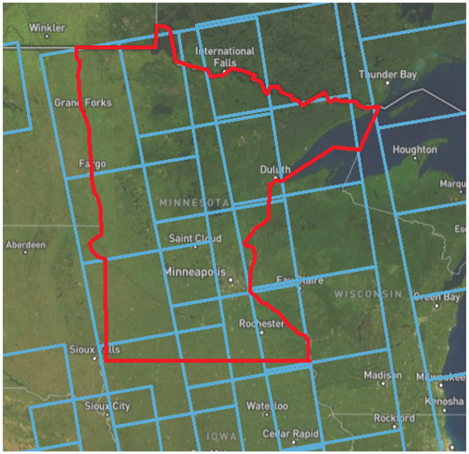
Distribution of SAR images over Minnesota.
To minimize seasonal variability, only summer acquisitions (June to August) were used, following guidance from previous SAR-C applications ( 27 ). Each image includes two polarization modes: VV (vertical transmit, vertical receive) and VH (vertical transmit, horizontal receive). Only VV was used in this study owing to its higher sensitivity to surface texture, making it more effective for detecting cracks, gaps, or other irregularities on paved surfaces ( 30 ).
Each Sentinel-1 scene was processed using the European Space Agency’s SNAP software ( 33 ), following procedures established during the development of the SAR-C tool ( 27 , 30 ). The workflow included orbit correction for accurate pixel geolocation, radiometric calibration to convert raw values to backscatter coefficients (γ0), speckle filtering using the intensity-driven adaptive-neighborhood method, and radiometric terrain correction to reduce terrain-related distortions. To minimize interference from transient features such as vehicles, pedestrians, or vegetation, annual image stacks were created, and the minimum γ0 value per pixel was extracted. This approach isolates stable surface conditions, as temporary objects typically produce higher and more variable backscatter ( 27 ).
Finally, the annual backscatter coefficient (

Sidewalk Data
This study used geospatial sidewalk data provided by MnDOT. These included two point-based datasets: the inspections dataset and the obstructions dataset, which include sidewalk locations across Minnesota with field measurements collected between 2018 and 2024.
The inspections dataset serves as the primary input for model development. It includes regularly spaced inspection points, approximately every 10 m, matching the 10- × 10-m resolution of the SAR imagery. This spatial alignment ensures consistency between satellite-derived features and ground-truth observations. Each point includes attributes such as sidewalk geometry, surface material, adjacent context, and condition rating using the scale illustrated in Figure 1.
Because the SAR pixel footprint is larger than the sidewalk surface, nearby features such as grass strips, paved boulevards, and curb ramps can influence the backscatter signal. In Minnesota, sidewalks are typically narrower than 10 m, so a substantial portion of the SAR return may originate from adjacent areas. If these materials are not considered, they can obscure signs of surface deterioration. As shown in Figure 5, the SAR pixel often captures both the sidewalk and the adjacent boulevard. To improve classification accuracy, attributes from both areas were included as input features in the model.
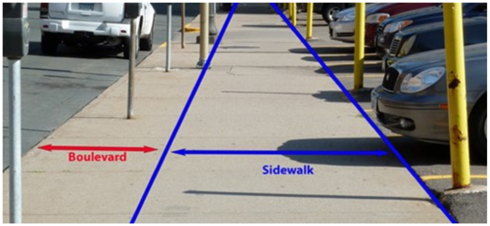
Visual representation of sidewalk and boulevard over a sidewalk segment.
To ensure the model can (a) capture how raw amplitude values vary between sidewalk locations, (b) account for the influence of surrounding features on those amplitude values, and (c) relate attributes to the actual sidewalk condition, the following attributes were selected for analysis:
Sidewalk width (measured in meters): This attribute corresponds to the width of the sidewalk measured at each inspection point.
Material: The surface material of the sidewalk (e.g., concrete versus asphalt) is an important feature because it affects the amplitude of the radar backscatter. Concrete generally returns a lower radar backscatter signal owing to its smoother finish, whereas asphalt tends to produce higher backscatter because of its higher roughness ( 34 ). By including material, the model can separate amplitude variations caused by inherent material properties from those caused by actual cracking or surface damage.
Sidewalk type: This feature is a categorical attribute describing the sidewalk function (e.g., pedestrian access route, shared-use path, driveway). Different sidewalk types may exhibit different wear patterns and expected levels of surface quality; incorporating this information helps the model interpret whether a given amplitude value corresponds to normal usage or to potential deterioration.
Crossing slope (%): This is the transverse slope of the sidewalk surface, measured perpendicular to pedestrian travel, recorded as an absolute percentage value. A steep crossing slope can deflect the radar signal away from the satellite sensor, altering the recorded amplitude. By including crossing slope, the model can correct for geometric effects that could otherwise be mistaken for changes in surface roughness.
Running slope (%): This attribute corresponds to the longitudinal slope, measured in the direction of pedestrian movement, and is recorded as an absolute percentage value. Because sidewalks often follow the roadway’s grade, running slope influences how water drains, which may affect deterioration over time.
Boulevard width (measured in meters): This feature characterizes the width of the buffer (grass, pavement, or landscaping) immediately adjacent to the sidewalk. In a 10-m pixel, a wide boulevard can occupy a significant portion of the pixel, causing most of the backscatter to originate from the boulevard rather than the sidewalk. By explicitly modeling boulevard width, the model can estimate how much of each pixel’s amplitude should be attributed to the boulevard versus the sidewalk itself.
Boulevard material: This attribute corresponds to the surface type adjacent to the sidewalk (e.g., grass, asphalt, pavers/brick). Different materials reflect radar signals differently. Grass typically yields lower backscatter, whereas asphalt or pavers produce higher backscatter. Knowing the material of the boulevard strip helps the model account for these differences in the SAR signal.
Condition rating: This is the target variable of the predictive algorithm, assigned according to MnDOT’s four-level scale (1 = good, 2 = fair, 3 = poor, 4 = severe). Sidewalk condition at each inspection point was determined by trained field staff based on standardized visual criteria. In later modeling experiments, an alternative binary classification (i.e., defective and nondefective) was explored to identify sidewalks requiring maintenance.
The obstructions dataset identifies sidewalk features that may interfere with pedestrian movement or affect SAR signal response. These georeferenced points are recorded only where obstructions exist and are not uniformly spaced. As shown in Figure 6, obstruction points (blue) are distinct from inspection points (red) and often represent vertical elements such as poles, signage, or utility boxes that can distort radar signals through a double-bounce effect. Obstructions were categorized into three groups: permanent (e.g., fixed infrastructure), temporary (e.g., short-term disruptions), and defective (e.g., broken or displaced pavement). A 10-m spatial join was used to associate each obstruction with its nearest inspection point. To ensure alignment, only matches sharing the same sidewalk segment identifier were retained.
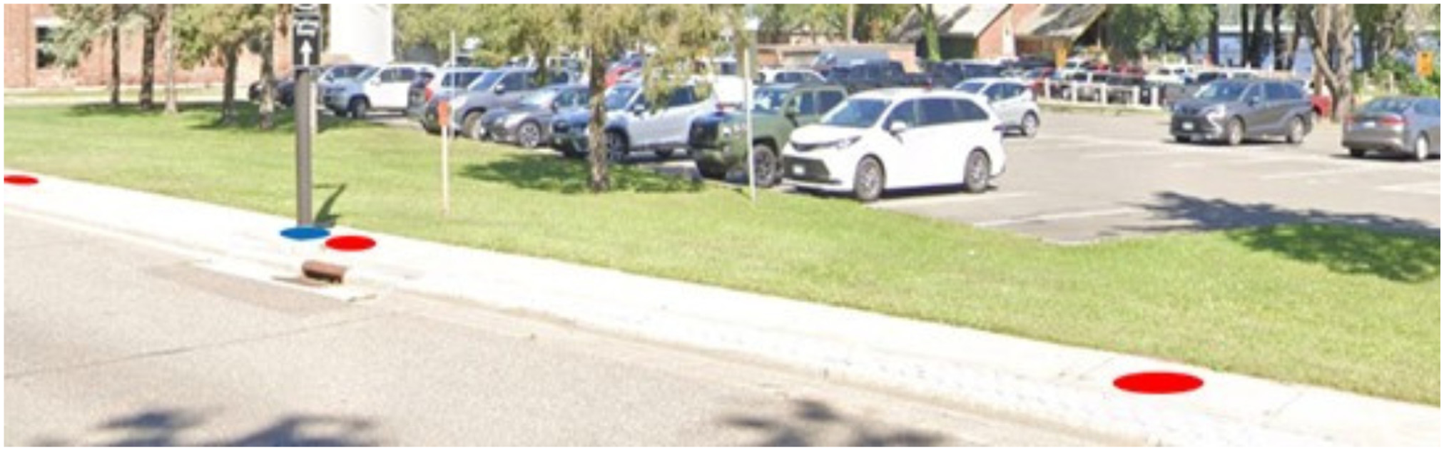
Representation of inspection point and obstruction point.
Figure 7 shows that points with permanent obstructions exhibit higher values of SAR amplitude and greater variability, compared with inspection points without obstructions. A Mann–Whitney U test was used to evaluate whether this difference was statistically significant. The test yielded a p-value less than 0.001, indicating that amplitude values were statistically larger in locations with permanent obstructions. This confirmed that such features introduce signal distortions that could mislead classification models. To address this issue, inspection points with permanent obstructions were removed from the analysis. Inspection points with temporary or defective obstructions were kept in the dataset. Additional filtering excluded roadway crossings and entries with missing or invalid data. This process reduced the initial dataset from 177,489 entries to 144,911 inspection points.
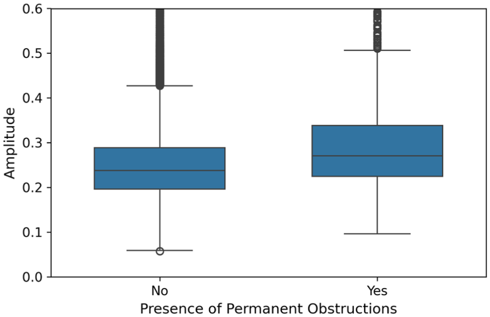
Effect of permanent obstructions on SAR amplitude.
Data Integration
The final set of inspection points was integrated with preprocessed SAR imagery to extract the corresponding backscatter amplitude. Although condition data were available from 2018 to 2024, two factors limited the number of usable inspection points. First, the failure of Sentinel-1B in late 2021 resulted in no available summer imagery from 2022 to 2024 ( 35 ). Inspection records from those years were excluded, reducing the dataset from 144,911 to 108,684 points. Second, 14,482 points from 2018 to 2021 were located outside the spatial extent of available SAR coverage and were therefore also removed. Considering this, a total of 91 SAR scenes collected between 2018 and 2021 were used in the study.
The resulting dataset includes 94,202 inspection points with complete ground-based attributes such as width, slope, surface material, boulevard characteristics, and condition rating. Each point also has a corresponding SAR amplitude value from the year it was inspected. Each inspection point was matched to the annual SAR amplitude composite value obtained for the same calendar year as the field inspection. Annual SAR amplitude composites were formed by stacking all summer (June to August) Sentinel-1 scenes within a given year and extracting the minimum γ0 value per pixel. This approach is meant to minimize the influence of transient features such as traffic and moisture, as demonstrated in previous work ( 27 ). For example, a sidewalk segment inspected in 2020 was paired with the 2020 summer composite. This matching strategy ensured temporal consistency between the satellite signal and ground-truth assessments. Field records from 2022 to 2024 were excluded because no usable summer Sentinel-1 imagery was available following the failure of Sentinel-1B in late 2021. This integrated dataset is referred to as the input dataset.
Machine Learning Model
Model Selection and Overview
A random forest classifier (Figure 8) was used as the machine learning algorithm. This algorithm maps the input dataset (i.e., Sentinel-1 backscatter amplitudes and sidewalk features) with condition categories. A random forest constructs an ensemble of decision trees, each trained on a random subset of inspection points and predictor variables. When using the algorithm to make predictions, each tree casts a vote, and the forest’s majority decision determines the final classification ( 36 ). By averaging over many trees, this method achieves better generalization than a single decision tree and reduces overfitting ( 37 ). Tuning this machine learning algorithm consists of selecting the number of trees, the maximum depth of each tree, and how many features to consider when splitting. An interesting feature of random forests is that they naturally produce feature-importance scores, which reveal how strongly each predictor influences the classification.
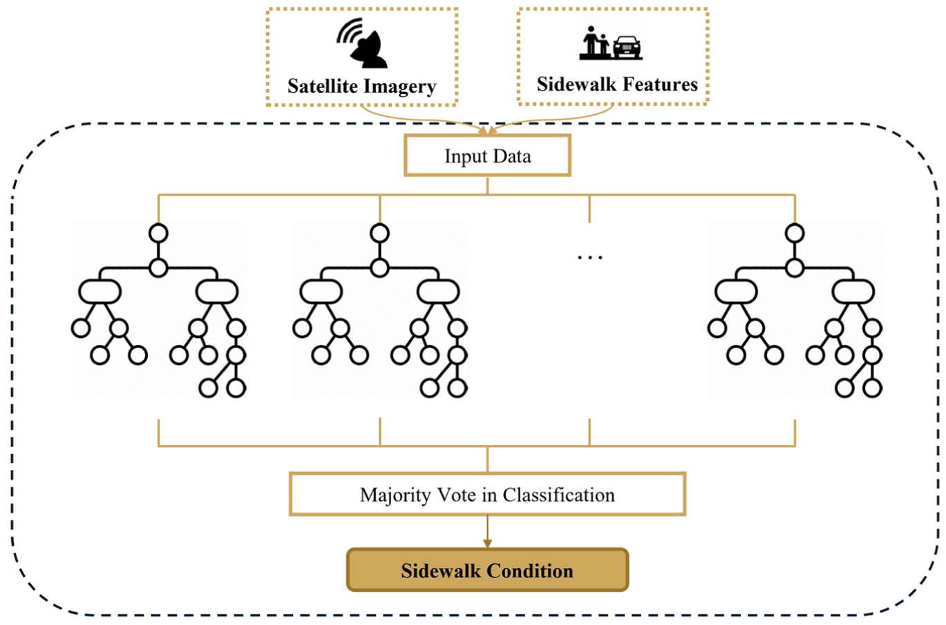
Random forest classifier was used to predict sidewalk condition rating.
To ensure that the random forest model would generalize well to unseen data, the input dataset was partitioned into training and test subsets. Eighty percent of the sidewalk segments were allocated to the training set whereas the remaining 20% was reserved as a test set to evaluate the performance of the model. Stratified sampling was used to maintain the original distribution of condition classes in both subsets. This approach prevents either the training or test set from becoming unbalanced in class proportions.
Imbalance in Condition Data
One of the challenges in modeling sidewalk condition is the imbalance of the dataset (Figure 9). Cases of class imbalance, where one class significantly outnumbers others, is a common issue in machine learning that can lead models to favor the majority class and overlook minority cases ( 38 ). In this study, 55.8% of inspections fell into Condition 2 (the majority class), whereas only 2.1% fell into Condition 4 (the minority class), yielding an imbalance ratio of 0.038.
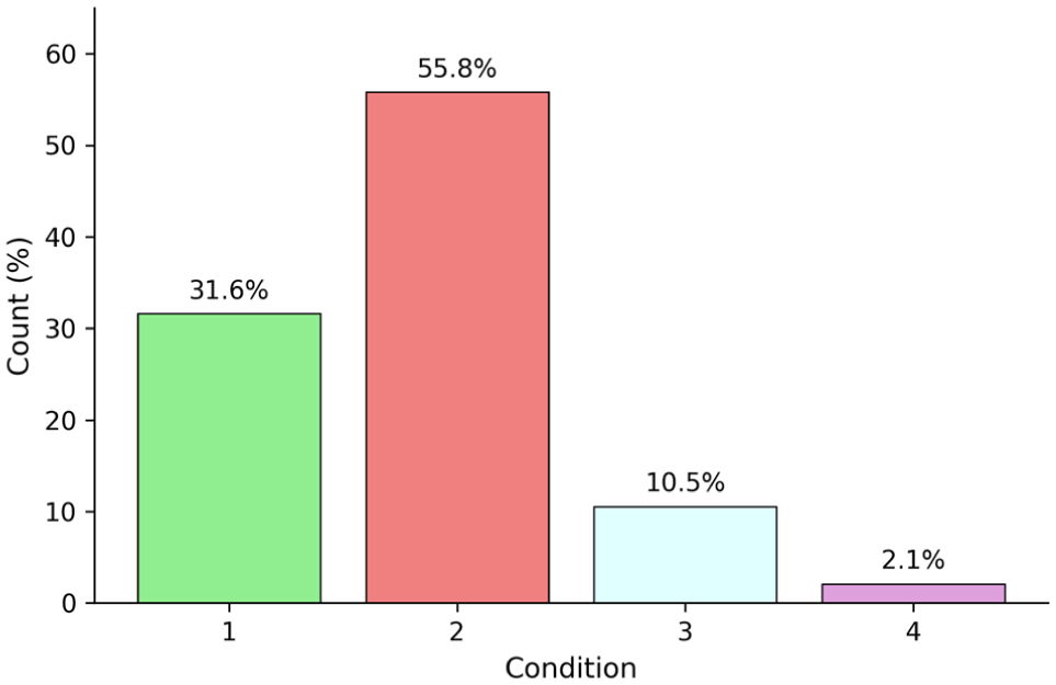
Distribution of sidewalk condition.
In this study, the imbalance ratio (IR) is defined as the ratio of minority class samples to majority class samples (IR = minority/majority), such that values closer to 1 indicate better balance. Some studies use the inverse definition (majority/minority), and both conventions are valid. Prior work shows that classification performance can become challenging even at moderate imbalance levels, with ratios around 1:10 already difficult to handle, and more extreme ratios such as 1:100 or higher representing severe imbalance conditions ( 39 ). With regard to IR, this corresponds approximately to values near 0.1 indicating moderate imbalance and values near 0.01 or lower indicating severe imbalance.
To prevent a classifier from simply learning to predict the majority class, two approaches were explored in this study: (1) reduce the number of classes and (2) consider under- and oversampling strategies. In particular, this study explored merging the two categories with the lowest-frequency (Conditions 3 and 4) into a “defective” class, and the two categories with highest frequency (Conditions 1 and 2) into a “nondefective” class. This process raised the IR to 0.144, bringing the minority and majority classes closer in size, which is preferable when training machine learning models.
Sampling Strategies to Reduce Imbalance
Even after merging the four condition levels into a binary scale, nondefective sidewalks remained the dominant class. To address this imbalance, a hybrid strategy combining Synthetic Minority Oversampling Technique (SMOTE) and random undersampling was applied. SMOTE generated synthetic examples of underrepresented segments (i.e., Conditions 3 and 4) to improve representation of the minority class, while random removal of nondefective samples (i.e., Conditions 1 and 2) was used as an undersample technique to reduce model bias. This approach ensured the random forest model could effectively learn from all classes ( 40 ).
Two sampling strategies were tested in both the four-class and binary classification models. Each case is labeled by classification type (“F” for four-class, “B” for binary) followed by a number indicating the strategy. In both models, a case with no resampling (labeled as F-0 and B-0) was used as a baseline. This case was compared with an alternative case consisting of a partial resampling that combined under- and oversampling (labeled as F-1 and B-1).
Validation and Performance Metrics
To evaluate model performance, a set of metrics suited for both binary and multiclass scenarios was used. These metrics assess not only overall prediction accuracy but also the model’s ability to identify the minority class, such as sidewalk segments in poor or defective condition, which is critical for maintenance planning.
Confusion matrices (such as the example shown in Figure 10) compare predicted and actual classifications and are commonly used to summarize model accuracy in classification problems. In the binary case (defective versus nondefective), the outcomes include counts of: true positive (TP), which represent the number of defective sidewalks correctly predicted as defective; true negative (TN), which account for the number of nondefective sidewalks correctly predicted as nondefective; false positive (FP), which corresponds to nondefective sidewalks incorrectly predicted as defective; and false negative (FN), which account for instances where defective sidewalks were incorrectly labeled as nondefective.
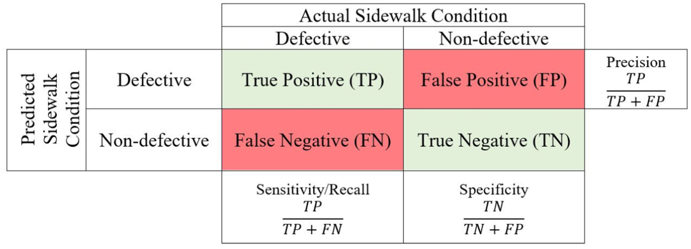
Confusion matrix of a binary model.
From these counts, the following metrics of performance can be estimated:
Precision: Measures the accuracy of the model’s positive predictions. It is calculated by dividing the number of TPs (correctly classified positive instances) by the total number of instances predicted as positive (TPs + FPs) (Equation 2). A hypothetical perfect model would have zero false positives and therefore a precision of 1.0. In this study, precision is calculated as the portion of sidewalk segments correctly predicted as defective, compared with all segments predicted as defective. Assuming that agencies only reevaluate points that the algorithm classifies as defective, high precision would make their work time-effective.

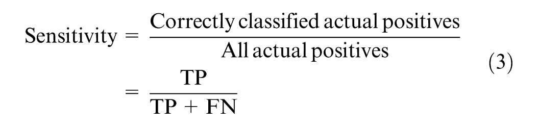
Sensitivity (or recall): Measures the proportion of all actual positives (in this study, defective segments) that were correctly classified as positives (i.e., defective) (Equation 3). A hypothetical perfect model would have zero FNs and therefore a recall of 1.0, which is to say, a 100% detection rate. In the context of sidewalk condition assessment, sensitivity is important because a model with high sensitivity/recall would detect all actually defective segments. In other words, high sensitivity/recall can be interpreted as the tool being reliable in detecting sidewalk segments in poor conditions.
G-mean: Overall metric of model performance that balances performance across classes. For binary classification, it is the geometric mean of sensitivity and specificity.
For binary classification:

where

Note that specificity equals the sensitivity or recall of the negative class.
For multiclass models, the geometric mean of sensitivity across all classes is used to calculate G-mean,

In the four-class model (good, fair, poor, and severe), precision and sensitivity are computed for each class, and G-mean is used to evaluate overall performance. Overall, the combined use of these metrics provides a comprehensive understanding of the model’s strengths and limitations, ensuring balanced attention to both frequent and rare sidewalk conditions.
Beyond their mathematical definition, these metrics have distinct practical implications for infrastructure management. Precision serves as a proxy for operational cost-efficiency: a higher precision minimizes the false alarms that waste inspector time and resources on nondefective segments. In contrast, recall (sensitivity) acts as a measure of safety and risk mitigation. In the context of ADA compliance and pedestrian safety, missing a severe defect (FN) presents a significant liability. Therefore, the G-mean was utilized to ensure that the model provided a balanced solution that maximizes resource efficiency without compromising the detection of critical safety hazards.
To quantify how much each input feature contributes to the model’s predictions, feature-importance analysis was performed for the model showing higher performance. This analysis was performed using the mean decrease in impurity (MDI), also referred to as Gini importance, which is the default feature-importance measure in the scikit-learn random forest classifier ( 41 ). For each feature, MDI measures the total reduction in node impurity weighted by the proportion of samples reaching each node, averaged across all trees in the forest. Higher MDI values indicate features that more consistently reduce classification uncertainty.
Results
Four-Level Classification
This section presents results for models trained on MnDOT’s original four-level sidewalk condition scale (1 = good, 2 = fair, 3 = poor, 4 = severe). Results are reported for two sampling strategies: a baseline model with no resampling (Case F-0) and a partially resampled model using a combination of undersampling and SMOTE (Case F-1). In Case F-1, Conditions 1 and 2 were each reduced to 15,000 samples through random undersampling, Condition 3 remained unchanged at 9,851 samples, and Condition 4 was expanded from 1,995 to 5,000 using SMOTE. This configuration yielded an IR of 0.33 between the smallest and largest classes. The class distribution in F-1 is shown in Figure 11, with lighter bars showing the data that were kept or synthetically added, and the darker bars depicting removed or expanded cases.
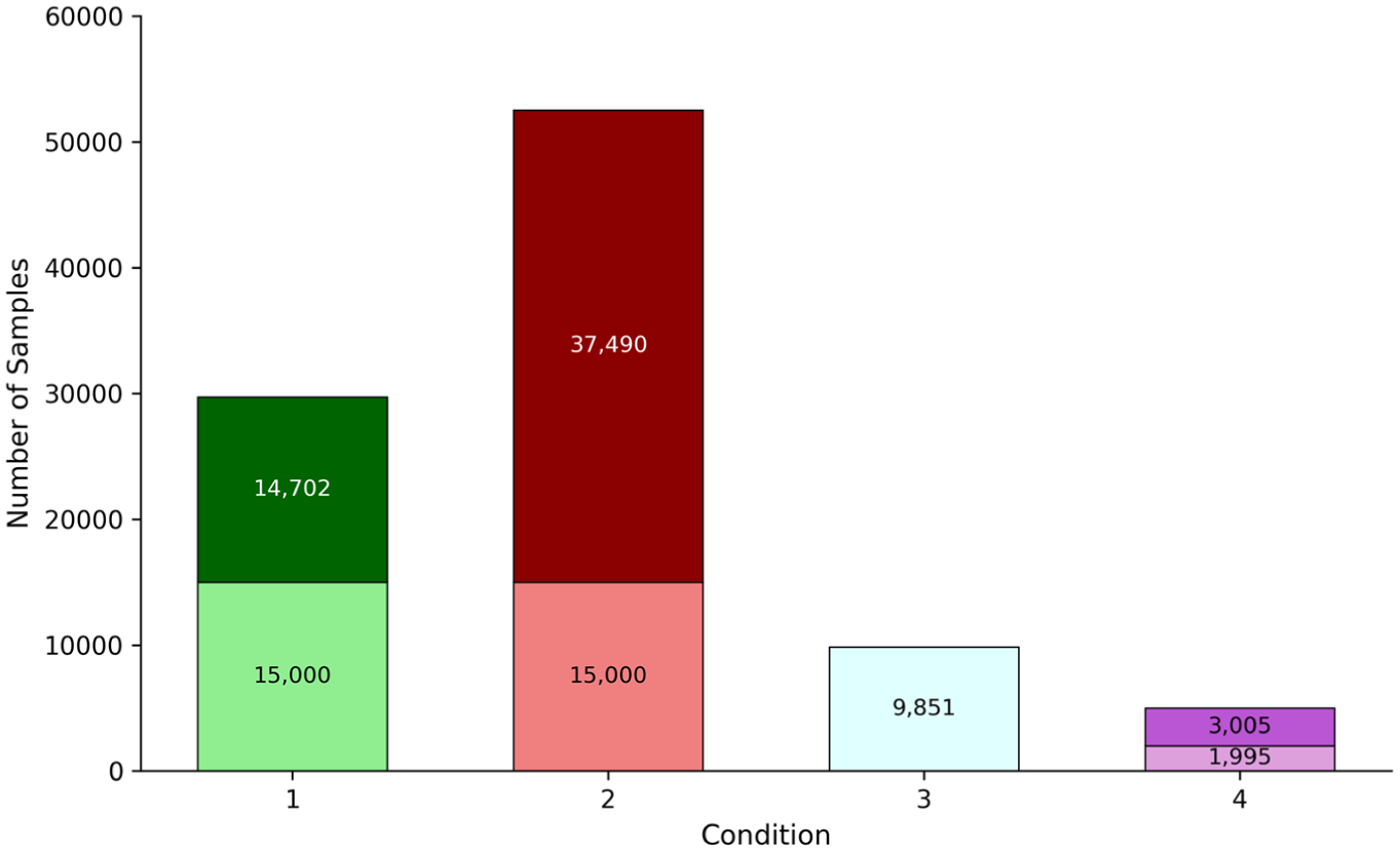
Data distribution for imbalanced sampling in Case F-1.
When using the dataset as is, without any resampling or class balancing (Case F-0), there is a risk of the model being biased toward predicting the most common categories and struggling to correctly identify the rare cases. This issue is illustrated in the confusion matrix (Figure 12a). Among all sidewalks labeled as Condition 1, the model correctly predicted 3,961 (67%) of them as “good.” However, 33% of sidewalks in good condition were misclassified: 1,846 (31%) were labeled as “fair,” 119 (2%) as “poor,” and 10 (∼0%) as “severe.” This shows that the model did reasonably well in predicting the most common class. Similarly, it correctly classified the majority of segments in Condition 2 (i.e., 8,516 out of 10,506 or 81% of segments were correctly classified). The accuracy of less frequent categories dropped significantly. Only 635 of 1,991 segments (i.e., 31%) in Condition 3 were correctly classified, whereas most (i.e., 53%) were mistakenly labeled as Condition 2. The situation was even worse for Condition 4, where only 123 out of the 375 cases (i.e., 33%) were correctly labeled and the rest were mainly predicted as Condition 2.
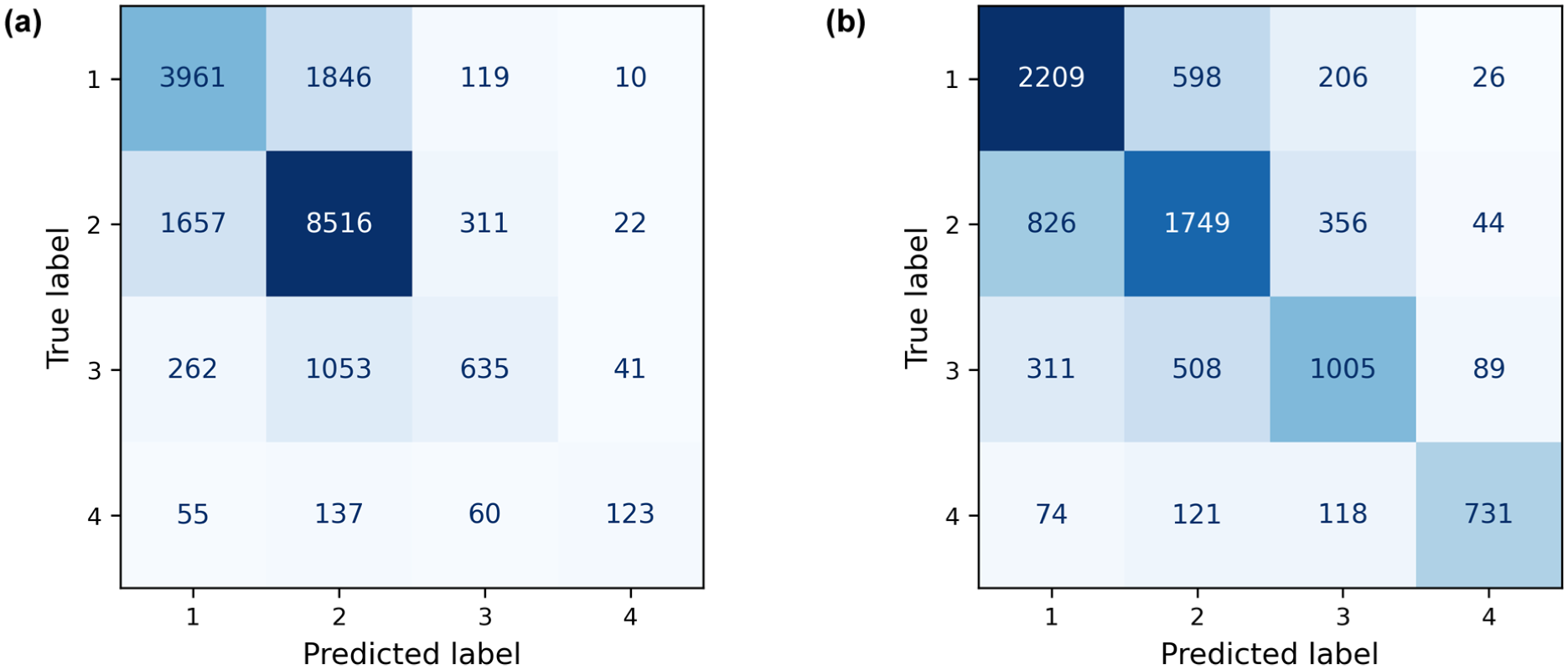
Confusion matrix with (a) no resampling (F-0) and (b) strategic sampling (F-1).
These results highlight the model’s bias toward the majority classes, which stems directly from the imbalance in the training dataset. The overwhelming number of Condition 2 examples during training caused the model to favor “fair” predictions, even for sidewalks in poor or severe condition. Consequently, the model struggled to detect deteriorated sidewalks, which are precisely the segments that are most in need of maintenance. This underscores the importance of addressing class imbalance to improve model fairness and ensure that sidewalks in poor condition are not overlooked.
The strategic combination of under- and oversampling (Case F-1) helped reduce class imbalance and enhance model accuracy. The confusion matrix in Figure 12b shows better results across all categories when compared with Case F-0 (Figure 12a). The model correctly predicted 2,209 of the 3,039 (i.e., 73%) Condition 1 samples and 1,749 of the 2,975 (i.e., 59%) Condition 2 samples. For Condition 3, the model correctly identified 1,005 cases out of 1,913 (i.e., 53%), and for Condition 4, it correctly predicted 731 out of 1,044 (i.e., 70%). These results suggest that the F-1 sampling strategy allowed the model to make accurate predictions for all four conditions, including the rare cases of severe condition, which are particularly critical for the appropriate management of these assets.
Table 1 summarizes key performance metrics (precision, sensitivity, and G-mean) for each of the four condition categories in the two sampling strategies (Case F-0 and Case F-1). When interpreting these data, it is important to keep in mind that a random predictor in a four-level model, which could serve as a baseline for comparison, would have precision, sensitivity, and G-mean values of 0.25. The proposed model significantly outperformed this random predictor.
Performance Summary of Four-Level Model
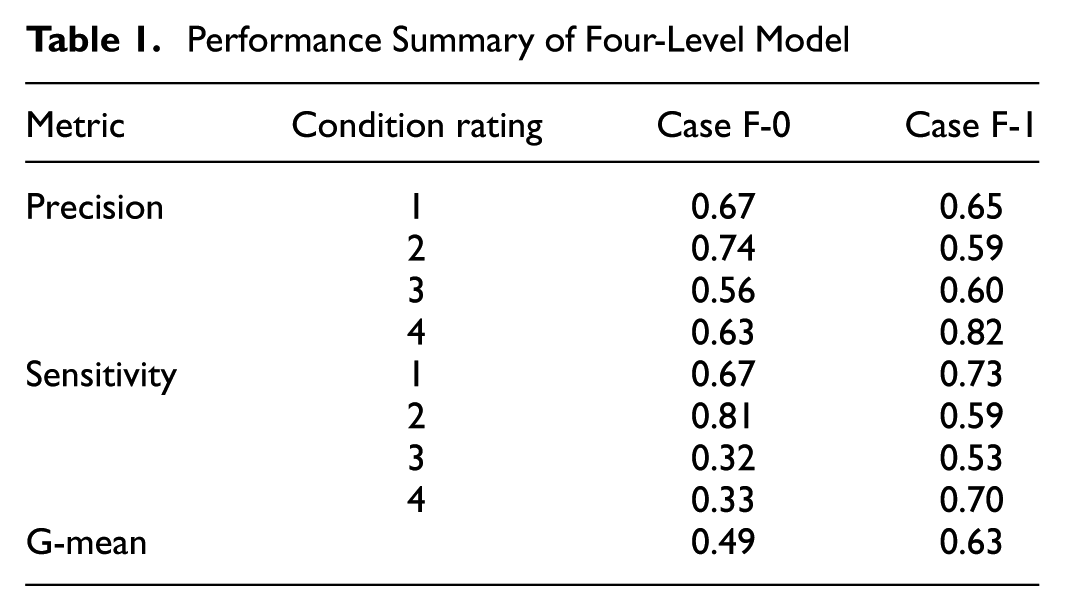
The baseline model trained on the original imbalanced dataset (Case F-0) showed strong bias toward the majority classes. Precision for Conditions 1 and 2 remained relatively high at 0.67 and 0.74, respectively, whereas Conditions 3 and 4 fell to 0.56 and 0.63. Sensitivity values further highlighted this imbalance: Condition 2 achieved 0.81, whereas Conditions 3 and 4 dropped to 0.32 and 0.33, respectively. As a result, the model rarely detected sidewalks in “poor” or “severe” condition, and the G-mean fell to 0.49, indicating weak overall balance in class prediction.
A targeted resampling strategy (Case F-1) resulted in performance improvements across all classes. Precision values increased for Conditions 3 and 4 to 0.60 and 0.82, respectively, whereas Conditions 1 and 2 were maintained at 0.65 and 0.59. Sensitivity values became more evenly distributed: 0.73 for Condition 1, 0.59 for Condition 2, 0.53 for Condition 3, and 0.70 for Condition 4. The balanced values of sensitivity across classes contributed to a G-mean of 0.63.
Compared with the baseline, Case F-1 demonstrated stronger performance in identifying both common and rare conditions. It improved recognition of sidewalk segments in poor and severe conditions without severely compromising the detection of more frequent cases, making it an effective strategy for classification in the four-level problem.
Binary Approach
To further explore options to reduce class imbalance, a binary classification was explored. Case B-0 represents the baseline binary classification model trained on the original, imbalanced dataset; whereas Case B-1 combined SMOTE to expand the defective class from 11,846 to 23,692 and the nondefective class was undersampled to match this figure and obtain an IR of 1 (Figure 13).
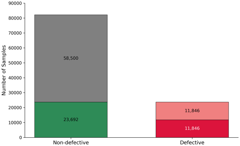
Data distribution of the combined approach for the binary model.
Similar to the results obtained in the four-level problem, the model trained on the original, imbalanced dataset was biased toward the majority class and struggled to identify defective sidewalks. As shown in the confusion matrix (Figure 14a), the B-0 model correctly identified 15,853 (i.e., 96%) nondefective sidewalks and 971 (i.e., 41%) defective sidewalks. Although, at first glance, the overall accuracy might seem high, owing to the dominance of nondefective cases, this masks the model’s poor performance on the class of greatest concern (i.e., defective sidewalks). The model, in fact, failed to detect a large portion of the defective class, misclassifying 1,395 (i.e., 59%) defective sidewalks as nondefective. This led to very low sensitivity for the defective category, meaning that many deteriorated sidewalks went undetected. Results obtained in Case B-0 highlight the need to consider resampling strategies to better balance the training data and improve the detection of sidewalks that require maintenance.
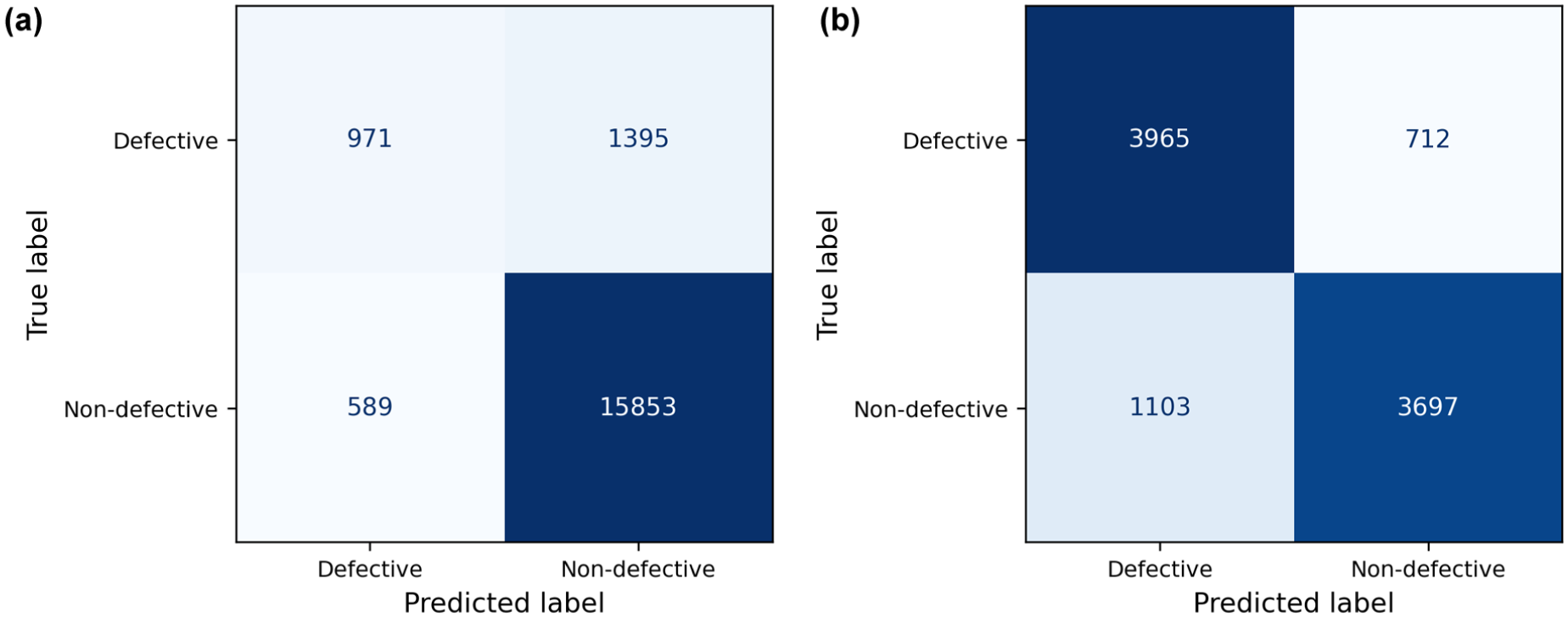
Confusion matrix with (a) no resampling (B-0) and (b) strategic sampling (B-1).
The model trained with a sampling strategy that combined over- and undersampling (Case B-1) resulted in improved performance in both classes (Figure 14b). The model correctly classified 3,965 (i.e., 85%) defective sidewalks and 3,697 (i.e., 77%) nondefective ones. Compared with the previous model, this represents a significant improvement in both sensitivity and precision for the defective class, while also maintaining strong performance for nondefective cases. Although there were still some misclassifications—712 (i.e., 15%) defective points labeled as nondefective and 1,103 (i.e., 23%) nondefective points labeled as defective—these errors were more evenly distributed and less severe than in the baseline (B-0) model.
Table 2 summarizes the key performance metrics, including precision, sensitivity, and G-mean for the two sampling strategies analyzed in the binary-scale problem (Cases B-0 and B-1). A random predictor in a binary model, which could serve as a baseline for comparison, would have precision, sensitivity, and G-mean values of 0.50. The proposed model significantly outperformed this random predictor.
Performance Summary of Binary Model
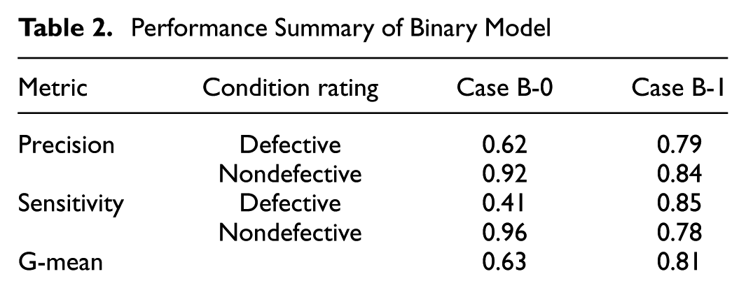
Case B-1, which combined under- and oversampling, improved recall for the defective class to 0.85 while maintaining a precision of 0.79. Performance on the nondefective class remained strong, with a precision of 0.84 and specificity of 0.78. The G-mean rose to 0.81, indicating a well-balanced model. In contrast, the baseline model (Case B-0) showed limited ability to identify defective sidewalks. Although precision for nondefective cases was high (0.92), recall for defective segments was just 0.41, resulting in a G-mean of only 0.63. These findings demonstrate the importance of addressing class imbalance during training to improve the model’s ability to detect minority cases while preserving overall performance.
Comparison of Binary and Four-Level Rating Scales
Based on the results, the binary model (Case B-1) showed a stronger performance than any of the four-level configurations, with a G-mean of 0.81, whereas the best four-level model (Case F-1) obtained a G-mean value of only 0.63. This improvement was probably owing to the binary approach significantly reducing class imbalance, making it easier for the model to learn and predict classes. In the binary setup, the model only needs to distinguish between “defective” and “nondefective” sidewalks, making it an easier classification problem that results in higher precision and sensitivity, especially for sidewalks in need of repair. However, the binary model has limited capabilities in distinguishing between different levels of deterioration. Although it flags whether a sidewalk is defective, it cannot differentiate between “poor” or “severe” categories. If detailed classification is needed for planning or prioritization, the four-level model remains relevant despite its lower accuracy. Although the four-level structure offered higher specificity, it performed worse overall, owing to imbalance issues and a greater likelihood of misclassification. It also required more aggressive sampling techniques, which may introduce bias or reduce data quality.
Feature-Importance Analysis
The analysis of feature importance (Figure 15) in Case F-1 found SAR amplitude to be the strongest individual predictor (MDI = 0.27), followed by running slope (MDI = 0.22), and crossing slope (MDI = 0.20). Although the two slope features were collectively more influential than amplitude (∼0.42 combined), no single geometric feature matched the stand-alone predictive contribution of the SAR-derived signal, confirming that amplitude captured surface roughness information that was not fully represented by the structural attributes of the sidewalk alone. In contrast, attributes such as surface material or the presence of temporary or defective obstructions made a lower contribution to the predictive ability of the model.
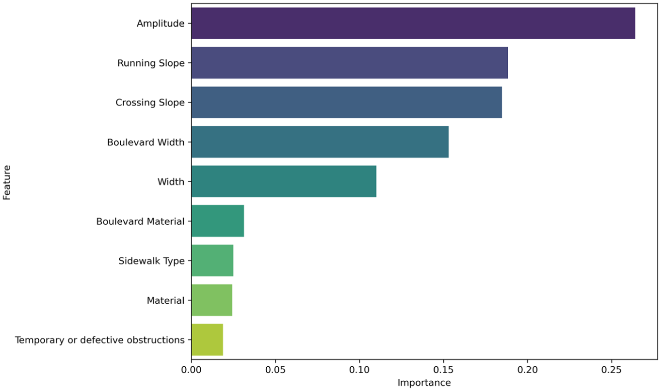
Feature importance in sidewalk condition prediction in Case F-1.
To further interpret the direction of each feature’s influence on condition, Figure 16 presents the mean values of the three key predictors by condition class. Defective sidewalks exhibited higher mean SAR amplitude (0.262 versus 0.255 for nondefective sidewalks), consistent with the physical expectation that surface deterioration produces increased roughness and therefore higher amplitude of radar backscatter. Among the geometric features, crossing slope showed the most pronounced directional pattern: sidewalks classified as defective had a mean crossing slope of 2.16%, compared with 1.83% for nondefective sidewalks, suggesting that steeper transverse grades were associated with worse condition, likely owing to accelerated drainage-related stress and repeated freeze–thaw cycles. Running slope showed a negligible difference between condition classes (1.533% versus 1.521%), suggesting that longitudinal grade did not independently drive deterioration in this dataset. Although these differences were found to be statistically significant using the Mann–Whitney U test (i.e., p-values < 0.01 for all three features), the effect size was found to be small (i.e., between 0.45 and 0.48), which allowed us to conclude that, in isolation, the effect of each of these features on sidewalk condition was negligible. The predictive power of the random forest classifier therefore comes from the combination of variables, rather than any single dominant feature.
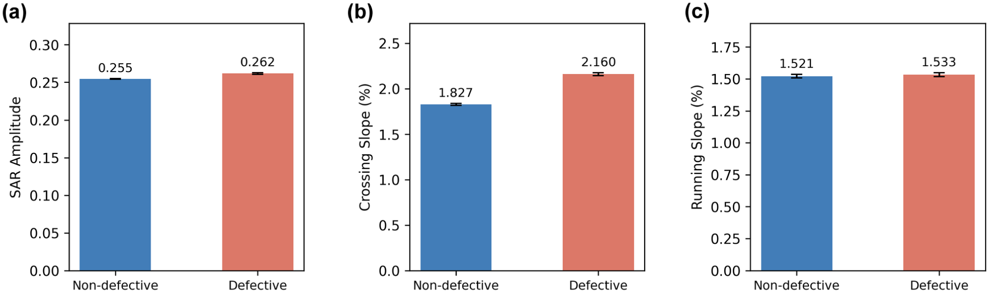
Mean values of key predictors by sidewalk condition class: (a) SAR amplitude, (b) crossing slope, and (c) running slope.
Although the example shown in Figure 15 is specific to Case F-1, similar results were obtained with other sampling strategies. This suggests that SAR data serve as significant predictors of surface deterioration, offering valuable information on sidewalk conditions even without field-based inspections. In contrast, attributes like surface material or the presence of temporary or defective obstructions made a lower contribution to the predictive ability of the model. This highlights the unique contribution of SAR data and their potential as a key input for future models analyzing surface conditions.
Conclusions
This study explored the potential of satellite SAR imagery and machine learning to assess sidewalk conditions. This task has traditionally relied on field inspections that are time-consuming. This study sought to provide MnDOT with a more scalable, consistent, and cost-effective method for monitoring sidewalk conditions.
Overall, this study showed that combining SAR imagery with machine learning can be a powerful and scalable tool for sidewalk condition assessment. This remote-sensing method is not meant to replace in-person inspections. It is instead conceived as a screening tool that could be used to point out potential deficiencies in the network that could then be evaluated by inspectors. This could assist public agencies in planning inspections and maintenance activities more efficiently, especially as pedestrian networks grow and budgets remain tight. This screening tool offers significant efficiencies. For example, manual condition assessments are time-consuming, often preventing frequent updates. Literature indicates that detailed condition assessments require significantly more time to complete than basic inventories ( 5 ). In Seattle, WA, manual inspection covered approximately 800 mi per month, whereas Pensacola, FL, and Sioux Falls, SD, recorded rates of approximately 360 and 225 mi per month, respectively ( 5 ). This difficulty in scaling manual methods results in infrequent data updates at the state level; a survey of 39 state DOTs found the required frequency for statewide sidewalk data collection was less than annually, with the majority reporting a schedule of more than a year ( 6 ). This operational challenge limits the ability of agencies to establish network-level deterioration models that require consistent, longitudinal data. In contrast, the SAR-based method ensures the availability of longitudinal data necessary for deterioration models, as its source, the Sentinel-1 satellite, offers a rapid 12-day revisit cycle, making continuous statewide monitoring and annual network assessment readily achievable.
The results suggest that class imbalance poses major challenges, especially when trying to predict rare but important cases of sidewalks in poor and severe conditions. To address this, a simpler binary classification model was explored. This model grouped the four original ratings into two categories: defective and nondefective. This shift allowed the model to concentrate on segments requiring maintenance, and the resulting predictive model showed improved performance. Strategic sampling strategies combining under- and oversampling were compared with models trained with the original dataset (with no resampling). This analysis resulted in a total of four models: Cases F-0 and B-0, which used four-level and binary classification, respectively, with no resampling; and Cases F-1 and B-1, which used strategic sampling in the four-level and binary problems, respectively.
A combination of under- and oversampling in the binary setting (Case B-1) showed the best results. This case considered a two-level classification (i.e., defective and nondefective sidewalks), used SMOTE to generate more samples of the rare class, and reduced the number of samples in the majority class. The model trained on this dataset achieved the highest sensitivity for defective sidewalks (0.85), and a high G-mean (0.81). These metrics showed that this model is both sensitive to deterioration and robust against bias caused by data imbalance.
Four-class models were also tested to maintain the detailed condition labels currently used by MnDOT. As expected, these models showed lower performance across evaluation metrics, which is typical in multiclass classification settings. This was partially because of the inherent difficulty in distinguishing between more categories, especially when some classes are underrepresented. Overall, the binary model proved to be effective for identifying sidewalks that need maintenance, making it a practical tool for near-term implementation.
The analysis of feature importance showed that SAR amplitude was the strongest predictor, followed by geometric features such as running slope and crossing slope. Attributes such as surface material or the presence of obstructions contributed less to the model’s predictions. This highlights the unique contribution of SAR data and their potential as a key input for future models analyzing surface conditions.
The reliance on a point-level train–test split presents a limitation in the validation strategy. This approach was chosen to enable stratified sampling, which was critical given the severe class imbalance (e.g., only ∼2% “severe” cases). Spatially blocked splitting posed a risk of excluding minority classes entirely from the test set. However, this point-level split did not account for spatial autocorrelation, as neighboring points may appear in both training and test sets. Although the high local variability of sidewalk defects means that neighboring points often have different condition ratings, the reported performance may still be influenced by spatial proximity. Future work implementing spatially blocked cross-validation (e.g., Leave-One-Group-Out) is recommended to rigorously test the potential for spatial autocorrelation and data leakage, which may inflate reported performance.
Additionally, the 10 m spatial resolution of Sentinel-1 resulted in mixed pixels where the sidewalk typically occupies around 20% of the satellite image pixel. Although the inclusion of boulevard attributes in the model mitigated this problem, higher resolution data could further improve precision. Future work is proposed to address these limitations by exploring high-resolution SAR imagery such as TerraSAR-X or COSMO-SkyMed ( 42 , 43 ). These sensors offer resolutions as fine as 1 m, reducing the mixed-pixel effect, though the trade-off between higher cost and accuracy gains must be evaluated against the scalability goals of public agencies.
Although a detailed financial return on investment (ROI) is outside the scope of this paper, the potential for high-value savings is clear. Future work could quantify this ROI by applying life-cycle cost frameworks that account for imperfect condition assessments, such as partially observable Markov decision process ( 44 ).
Footnotes
Acknowledgements
The authors are grateful for the financial support provided by the Minnesota Department of Transportation to develop this research project, and from the College of Engineering & Applied Sciences at the University of Colorado Boulder. They also express their gratitude for the guidance and constructive feedback received from the project manager (Michelle Pasko) and the study panel.
Author Contributions
The authors confirm contribution to the paper as follows: study conception and design: P. Ferrer-Font, I. Rahman, C. Torres-Machi; data collection: P. Ferrer-Font, I. Rahman; analysis and interpretation of results: P. Ferrer-Font, I. Rahman, C. Torres-Machi; draft manuscript preparation: P. Ferrer-Font, I. Rahman, C. Torres-Machi. All authors reviewed the results and approved the final version of the manuscript.
Declaration of Conflicting Interests
The authors declared no potential conflicts of interest with respect to the research, authorship, and/or publication of this article.
Funding
The authors disclosed receipt of the following financial support for the research, authorship, and/or publication of this article: This work was supported by the Minnesota Department of Transportation (MnDOT Contract Number: 1054249) and the College of Engineering & Applied Sciences at the University of Colorado Boulder through the Europe-Colorado Program.

Data Availability Statement
The datasets generated during and/or analyzed during the current study are available from the corresponding author on request.