Jackknife empirical likelihood confidence regions for the evaluation of continuous-scale diagnostic tests with verification bias

Abstract

Recently, Wang and Qin proposed various bias-corrected empirical likelihood confidence regions for any two of the three parameters, sensitivity, specificity, and cut-off value, with the remaining parameter fixed at a given value in the evaluation of a continuous-scale diagnostic test with verification bias. In order to apply those methods, quantiles of the limiting weighted chi-squared distributions of the empirical log-likelihood ratio statistics should be estimated. In order to facilitate application and reduce computation burden, in this paper, jackknife empirical likelihood-based methods are proposed for any pairs of sensitivity, specificity and cut-off value, and asymptotic results can be derived accordingly. The proposed methods can be easily implemented to construct confidence regions for the evaluation of continuous-scale diagnostic tests with verification bias. Simulation studies are conducted to evaluate the finite sample performance and robustness of the proposed jackknife empirical likelihood-based confidence regions in terms of coverage probabilities. Finally, a real case analysis is provided to illustrate the application of new methods.

Keywords

empirical likelihood estimating equations jackknife receiver operating characteristic verification bias

1 Introduction

Sensitivity and specificity are commonly used measures for evaluating the diagnostic accuracy of a test. If we use T as the continuous-scale test result for both diseased and non-diseased groups, and let D be the disease indicator with 1 as the diseased patient and 0 as the non-diseased patient, then, for a given cut-off level τ, the sensitivity θ and the specificity η of the test can be defined as follows

θ (τ) = P (T > τ | D = 1), η (τ) = P (T \leq τ | D = 0) .

The plot of sensitivity against 1-specificity is called the receiver operating characteristic (ROC) curve as the cut-off level τ varies.

In medical diagnostics, physicians would like to have the true disease status verified for every patient by applying a gold standard evaluation, which assesses disease status with certainty based on preliminary screening test results. However, in many situations, not all patients given their screening test results are willing to have their true disease status verified, due to various reasons. For example, gold standard tests may be unaffordable, time consuming, or too invasive. Usually, patients with positive test results are more likely to take a gold standard evaluation than patients with negative test results. If the decision of whether or not to have true disease status verified depends on screening test results and some other external factors, the evaluation of a screening test using sensitivity and specificity could be biased. This type of bias is verification bias¹ or work-up bias.² Verification-biased data can sometimes be assumed to be missing at random (MAR),^3,4 in which the probability that a patient has his or her disease status verified only depends on the screening test result and the patient’s observed characteristics. Alonzo and Pepe⁵ studied various bias-corrected ROC analyses based on estimating equations. Although the MAR assumption has been well studied, it is difficult to justify and stronger than the missing not at random (MNAR) assumption. Before applying the methods developed here, some preliminary works are necessary to check the potential missing mechanism.

Empirical likelihood (EL)^6–8 is a popular nonparametric method well known for its nice small sample performance. Chen and Van Keilegom⁹ provided a general review on EL method for regression models, pointing out that EL-based confidence regions would offer better confidence regions than the ones provided by asymptotic normality in small sample cases. Moreover, the shapes of EL-based confidence regions are data driven, while for normal approximation-based methods, the shapes of confidence regions are predetermined. Recently, motivated by Adimari and Chiogna,¹⁰ which considered joint confidence regions without missing data, Wang¹¹ and Wang and Qin¹² developed various bias-corrected joint EL confidence regions for continuous-scale tests. Their methods are based on the inverse probability weighting (IPW) estimator, the full imputation (FI) method, the mean score imputation (MSI) method, and the semi-parametric efficient estimator (SPE) for sensitivity and specificity. They constructed confidence regions for the pairs of (sensitivity, cut-off level), (specificity, cut-off level), and (sensitivity, specificity) based on limiting weighted chi-squared distributions of the empirical log-likelihood ratio statistics for sensitivity, specificity, and cut-off level. Also, they pointed out the necessity of constructing joint confidence regions. Their EL-based confidence regions provide visual tools to choose cut-off levels for desirable sensitivity and specificity by drawing contours of joint confidence regions for (θ, τ) and (η, τ) in the same graph. Such visual tools are easy to implement. Additionally, their proposed confidence regions have many of the same advantages as that of the EL method.

Jackknife EL method, prompted by Jing et al.,¹³ is a powerful EL-based method to overcome the computational difficulty associated with nonlinear functionals, with a particular application to U-statistics. Li et al.¹⁴ proposed a jackknife EL method to construct confidence regions for parameters of interest in the presence of nuisance parameters. With jackknife pseudo samples, the resulting jackknife EL method retains the attractive property of having standard chi-square limiting distributions. In order to reduce the computational burden in the jackknife EL method when explicit estimators of the nuisance parameters are unavailable, Peng¹⁵ proposed an approximate jackknife EL method. As argued by Adimari and Chiogna,¹⁶ the jackknife EL does not retain all features of the EL function because it is not a genuine EL function. To be specific, the jackknife EL-based confidence intervals and regions may not be range preserving. If this situation happens, the methods developed in Ref. [12] based on profile EL can still be applied.

In this paper, we apply jackknife EL methods to the framework proposed by Wang and Qin^11,12 to construct jackknife EL confidence regions for the evaluation of continuous-scale diagnostic tests in the presence of verification bias. Since the proposed jackknife empirical log-likelihood ratio statistics have standard chi-squared distributions as their asymptotic distributions, it is convenient to do joint inferences for sensitivity, specificity, and cut-off level. Most previous works, like Alonzo and Pepe,⁵ require estimates of complicated variance–covariance matrices based on normal approximation theory in order to do joint inferences. If explicit formulas for variance–covariance matrices are unavailable, bootstrap methods are required at a price of higher computational burdens. Also, Alonzo and Pepe⁵ used a large sample size, n = 5000, in their simulation studies, which are often unavailable. Our method retains the attractive properties of EL method: (1) having standard chi-squared distributions as asymptotic distribution of the EL ratio statistics, (2) avoiding estimation of any variance–covariance matrix. Additionally, our method works well with sample size $n \geq 300$ as shown in simulation studies, which in turn saves money and other resources.

We organize the paper as follows: section 2 uses the jackknife EL method to construct joint EL-based confidence regions in the presence of verification bias under an estimating equation framework, section 3 presents some simulation studies to evaluate the finite sample performance and robustness of the proposed method, and section 4 presents real data analysis with one data set. In section 5, a brief discussion is provided. In order to facilitate adoption of our method, we are pleased to offer sample R codes for the computation of the confidence regions.

2 Jackknife empirical likelihood confidence regions in the presence of verification bias

In the following, we use T_i to denote the continuous-scale test result from a screening test, and D_i to denote the dichotomous indicator of disease status without measurement error, for $i = 1, \dots, n$ , where D_i = 1 means the ith patient is diseased and D_i = 0 means the ith patient is free of disease. Let V_i denote the dichotomous indicator of verification status of the ith patient, with V_i = 1 if the ith patient has his or her true disease status verified, and V_i = 0 if otherwise. Usually, during the diagnostic process, some covariates, like demographic variables, are collected. By incorporating this information, it is possible to model the verification status, V_i’s, and disease status, D_i’s. Let A_i denote a vector of the observed covariates for the ith patient that may be associated with both D_i and V_i.

Similar to Refs. [11] and [12], we assume that the verification of disease status is conditionally independent of the true disease status given test results and observed covariates, i.e. $V ⊥ D | T, A$ . That is to say, whether or not a patient has his or her true disease status verified only depends on T and A regardless of the true disease status D, part of which are missing. Throughout this paper, all results are based on this assumption.

With i.i.d. samples S_i = (T_i, A_i, V_i, D_i) and the conditional independence of V_i and D_i given T_i and A_i, motivated by the IPW, FI, MSI, and SPE method-based bias-corrected estimators of sensitivity and specificity provided in Ref. [5], Wang¹¹ and Wang and Qin¹² provided following four pairs of estimating functions for $ϑ = (θ, η, τ)'$ , where always one component of ϑ is fixed

IPW : {g IPW, 1 (S i, ϑ, π i) = π_{i}^{- 1} V i D i (I (T i \leq τ) - (1 - θ)) g IPW, 2 (S i, ϑ, π i) = π_{i}^{- 1} V i (1 - D i) (I (T i \leq τ) - η) FI : {g FI, 1 (S i, ϑ, ρ i) = ρ i (I (T i \leq τ) - (1 - θ)) g FI, 2 (S i, ϑ, ρ i) = (1 - ρ i) (I (T i \leq τ) - η)

MSI : {g MSI, 1 (S i, ϑ, ρ i) = (V i D i + (1 - V i) ρ i) (I (T i \leq τ) - (1 - θ)) g MSI, 2 (S i, ϑ, ρ i) = (V i (1 - D i) + (1 - V i) (1 - ρ i)) (I (T i \leq τ) - η) SPE : {g SPE, 1 (S i, ϑ, π i, ρ i) = (V i D i / π i - (V i - π i) ρ i / π i) (I (T i \leq τ) - (1 - θ)) g SPE, 2 (S i, ϑ, π i, ρ i) = (V i (1 - D i) / π i - (V i - π i) (1 - ρ i) / π i) (I (T i \leq τ) - η)

where

π i = P (V i = 1 | T i, A i)

, and

ρ i = P (D i = 1 | T i, A i)

. Let

g IPW (S i, ϑ, π i) = (g IPW, 1 (S i, ϑ, π i), g IPW, 2 (S i, ϑ, π i))'

(2.1)

g FI (S i, ϑ, ρ i) = (g FI, 1 (S i, ϑ, ρ i), g FI, 2 (S i, ϑ, ρ i))'

(2.2)

g MSI (S i, ϑ, ρ i) = (g MSI, 1 (S i, ϑ, ρ i), g MSI, 2 (S i, ϑ, ρ i))'

(2.3)

g SPE (S i, ϑ, π i, ρ i) = (g SPE, 1 (S i, ϑ, π i, ρ i), g SPE, 2 (S i, ϑ, π i, ρ i))' .

(2.4)

If $π i$ ’s and ρ_i’s are known, by following a routine technique defining EL with estimating equations given by Qin and Lawless,¹⁷ inferences of unknown parameters could be done. However, $π i$ ’s and ρ_i’s are often unknown, and they turn out to be nuisance parameters. One popular way to get rid of these nuisance parameters is to replace them by their consistent estimators from parametric models on observed information, resulting in profile EL for ϑϑ.

Usually, logistic regression and probit models are employed to model $π i$ ’s and ρ _i ’s. Let $Z i = (1, T i, A i)', α = (α 0, α 1, α 2')', β = (β 0, β 1, β 2)'$ , and $Φ (\cdot)$ be the standard normal distribution function. For illustration, a probit model, $ρ i = Φ (Z i' α)$ , is used to model ρ _i ’s, and a logistic regression model, $π i = 1 / (1 + e - Z i' β)$ , is used to model $π i$ ’s by incorporating covariates Z_i’s. In estimating equation framework, for the probit model

Q 2 n, 1 (α) \equiv \frac{1}{n} \sum_{i = 1}^{n} V i Q 2, 1 (S i, α) \equiv \frac{1}{n} \sum_{i = 1}^{n} \frac{V i [D i - Φ (Z i' α)] φ (Z i' α)}{Φ (Z i' α) (1 - Φ (Z i' α))} Z i

(2.5)

is the estimating function for α, where exact disease statuses D_i’s are only available for verified subjects with V_i = 1 and

φ (\cdot)

is the standard normal density function. For the logistic regression model

Q 2 n, 2 (β) \equiv \frac{1}{n} \sum_{i = 1}^{n} Q 2, 2 (S i, β) \equiv \frac{1}{n} \sum_{i = 1}^{n} (V i - \frac{1}{1 + e - Z i' β}) Z i

(2.6)

is the estimating function for β.

If above models are correctly specified, we can obtain consistent estimates $\overset{\land}{α}$ of α and $\overset{\land}{β}$ of β. Then, profiled estimating equations are given by plugging in resulting consistent estimates $\overset{\land}{ρ} i = ρ (Z i, \overset{\land}{α})$ of ρ _i and $\overset{\land}{π} i = π (Z i, \overset{\land}{β})$ of $π i$ into equations (2.1) to (2.4). These plug-in estimating equations are easy to obtain, but they are not independent anymore. Therefore, Wang¹¹ and Wang and Qin¹² defined a plug-in EL for $ϑ = (θ, η, τ)'$ , and proved that the corresponding profile EL ratio statistics have weighted chi-squared distributions as their asymptotic distributions. Yet, the weights are required to be estimated before constructing confidence regions.

Motivated by Li et al.,¹⁴ the jackknife technique can be employed to obtain a standard asymptotic chi-squared distribution for the empirical log-likelihood ratio statistic of ϑ. Let $\overset{\land}{α} - i$ denote the solution to the equations

Q 2 n, - i, 1 (α) \equiv \frac{1}{n - 1} \sum_{j = 1, j \neq i}^{n} \frac{V j [D j - Φ (Z j' α)] φ (Z j' α)}{Φ (Z j' α) (1 - Φ (Z j' α))} Z j

(2.7)

and

\overset{\land}{β} - i

denote the solution to the equations

Q 2 n, - i, 2 (β) \equiv \frac{1}{n - 1} \sum_{j = 1, j \neq i}^{n} (V j - \frac{1}{1 + e - Z j' β}) Z j .

(2.8)

Set

T n, IPW (ϑ) = \frac{1}{n} \sum_{i = 1}^{n} g IPW (S i, ϑ, \overset{\land}{π} i) T n, FI (ϑ) = \frac{1}{n} \sum_{i = 1}^{n} g FI (S i, ϑ, \overset{\land}{ρ} i) T n, MSI (ϑ) = \frac{1}{n} \sum_{i = 1}^{n} g MSI (S i, ϑ, \overset{\land}{ρ} i) T n, SPE (ϑ) = \frac{1}{n} \sum_{i = 1}^{n} g SPE (S i, ϑ, \overset{\land}{π} i, \overset{\land}{ρ} i) .

And let $\overset{\land}{ρ} j, - i = Φ (Z j' \overset{\land}{α} - i)$ , $\overset{\land}{π} j, - i = \frac{1}{1 + e - Z j' \overset{\land}{β} - i}$ , for $j \neq i$ . Similarly, define

T n, - i, IPW (ϑ) = \frac{1}{n - 1} \sum_{j = 1, j \neq i}^{n} g IPW (S j, ϑ, \overset{\land}{π} j, - i) T n, - i, FI (ϑ) = \frac{1}{n - 1} \sum_{j = 1, j \neq i}^{n} g FI (S j, ϑ, \overset{\land}{ρ} j, - i) T n, - i, MSI (ϑ) = \frac{1}{n - 1} \sum_{j = 1, j \neq i}^{n} g MSI (S j, ϑ, \overset{\land}{ρ} j, - i) T n, - i, SPE (ϑ) = \frac{1}{n - 1} \sum_{j = 1, j \neq i}^{n} g SPE (S j, ϑ, \overset{\land}{π} j, - i, \overset{\land}{ρ} j, - i) .

Then, jackknife pseudo samples can be defined as follows

Y i, IPW (ϑ) = nT n, IPW (ϑ) - (n - 1) T n, - i, IPW (ϑ)

(2.9)

Y i, FI (ϑ) = nT n, FI (ϑ) - (n - 1) T n, - i, FI (ϑ)

(2.10)

Y i, MSI (ϑ) = nT n, MSI (ϑ) - (n - 1) T n, - i, MSI (ϑ)

(2.11)

Y i, SPE (ϑ) = nT n, SPE (ϑ) - (n - 1) T n, - i, SPE (ϑ) .

(2.12)

With similar argument in Tukey,¹⁸ the above $Y i, IPW (ϑ)$ ’s, $Y i, FI (ϑ)$ ’s, $Y i, MSI (ϑ)$ ’s, and $Y i, SPE (ϑ)$ ’s, $i = 1, \dots, n$ , are expected to be asymptotically independent, respectively. Then, the standard EL method can be applied to above jackknife pseudo samples for constructing joint EL confidence regions for ϑ. We define the jackknife EL function as follows

L J (ϑ) = sup {Π_{i = 1}^{n} p i : each p i > 0, \sum_{i = 1}^{n} p i = 1, \sum_{i = 1}^{n} p i Y i (ϑ) = 0}

(2.13)

where

Y i (ϑ)

could be any one of

Y i, IPW (ϑ), Y i, FI (ϑ), Y i, MSI (ϑ)

, and

Y i, SPE (ϑ)

. Using Lagrange multiplier method, the jackknife empirical log-likelihood ratio for ϑ is given by

l J (ϑ) = 2 \sum_{i = 1}^{n} \log (1 + \overset{\land}{t}' Y i (ϑ))

(2.14)

where

\overset{\land}{t}

is the solution of the following equation

\frac{1}{n} \sum_{i = 1}^{n} \frac{Y i (ϑ)}{1 + t' Y i (ϑ)} = 0 .

Theorem 1

Assume that $ϑ 0 = (θ 0, η 0, τ 0)$ is the true value of ϑ. Then

l J (ϑ 0) \to d χ_{2}^{2}

(2.15)

where

χ_{2}^{2}

is a chi-squared random variable with two degrees of freedom.

Remark 1

Theorem 1 can be proved by applying Theorem 1 in Ref. [14]. Conditions (A1) to (A7) in Ref. [14] should be verified. First, two points are noted. In our case, estimating equations $Q 2 n, 1 (α)$ for α and $Q 2 n, 2 (β)$ for β do not involve ϑ, so their estimates are not functions of ϑ. Additionally, the number of total parameters equals the number of estimating functions in our case, thus as mentioned in Ref. [14], $l J (\overset{\land}{ϑ}) = 0$ . We assume some regularity conditions on covariates, and $π i$ and ρ _i are bounded away from 0 and 1. Then all required conditions of the estimating equations containing main parameters can be verified. Also, conditions on the estimating equation containing nuisance parameters should be imposed. If a logistic or probit regression is considered, these conditions are naturally satisfied. Theorem 1 provides $l J (ϑ) = l J (θ, η, τ)$ as a good asymptotic pivot for the inference of the parameter pairs $(θ 0, τ 0), (η 0, τ 0)$ , or $(θ 0, η 0)$ with verification-biased data, when the third remaining parameter is fixed at a given value. Based on Theorem 1, we do not need to estimate any complex variance–covariance matrices, which are necessary for normal approximation-based inference. The complexity of estimating variance–covariance matrices limits the application of normal approximation-based methods, and bootstrap methods are often required as an alternative at a price of increased computational burden and time. For example, Alonzo and Pepe⁵ sketched the proof of asymptotic results in their framework of general estimating equations, and the formulas for their variance–covariance matrices were complicated. Therefore, they used a bootstrap method to estimate their variance–covariance matrices in their simulation studies.

Remark 2

Theorem 1 provides four types of bias-corrected joint confidence regions, which accommodate many situations. One could use one or several of them according to a specific situation. Also, simulation studies show that our methods work well with sample sizes, $n \geq 300$ , compared with n = 5000 in Ref. [5]. Therefore, in practice, this may result in saving money, time, and other resources.

Based on the above remarks and our simulation results in the next section, we can say that our method is the best one so far at hand for constructing joint confidence regions in the presence of verification bias under the MAR assumption.

In practice, the verification status is sometimes known. If this is true, it is unnecessary to apply IPW-based jackknife EL confidence regions for ϑ. One can use the simplified EL confidence regions for ϑ provided in Refs. [11] and [12] because the simplified empirical log-likelihood ratio statistic for ϑ is still a standard chi-square distribution with 2 degrees of freedom.

In this paper, we consider three types of $(1 - α) 100 %$ jackknife EL confidence regions as follows

$R α, 1 (θ, τ) = {(θ, τ) : l J (θ, η 0, τ) \leq χ_{α, 2}^{2}}$ ;

$R α, 2 (η, τ) = {(η, τ) : l J (θ 0, η, τ) \leq χ_{α, 2}^{2}}$ ;

$R α, 3 (θ, η) = {(θ, η) : l J (θ, η, τ 0) \leq χ_{α, 2}^{2}}$ ;

where

α \in (0, 1)

, and

χ_{α, 2}^{2}

is the

(1 - α)

-th quantile of the chi-square distribution with 2 degrees of freedom. Compared with the methods proposed in Refs. [11] and [12], we do not need to estimate quantiles of the weighted sum of the chi-square distributions. The method proposed in this paper gains from the application of jackknife technique. Thus, it brings more convenience in application.

The above three types of confidence regions will be utilized to choose a reasonable cut-off level for a continuous-scale test, where a reasonable cut-off level may generate balanced sensitivity and specificity, depending on researcher’s interest. It is noted that the issue of selecting an optimal cut-off based on a certain criterion is not addressed here, because it is beyond the scope of this paper. If the Youden Index is chosen as the criterion, it is a challenging task to obtain a good confidence interval of a selected optimal cut-off level, and bootstrap was the only method suggested by several recent studies through extensive simulations.^19–22 Instead, our confidence regions can show how the cut-off is related to the sensitivity/specificity when fixing specificity/sensitivity. Later in this paper, selecting a reasonable cut-off level will be illustrated by real data analysis. With the selected cut-off level, joint confidence regions of sensitivity and specificity can be constructed.

3 Simulation studies

In this section, simulation studies are conducted to evaluate the finite sample performance and robustness of the proposed various bias-corrected jackknife EL confidence regions.

Well-accepted model settings used in Ref. [5] are also employed in this paper for the purpose of comparison. First, two independent underlying continuous disease processes are generated, denoted by $Z 1 ~ N (0, 0.5)$ and $Z 2 ~ N (0, 0.5)$ . The disease status indicator D is generated as a binary variable: if a random variable $Z = Z 1 + Z 2 ~ N (0, 1)$ exceeds a certain threshold h, then D = 1, indicating the patient is diseased; otherwise, D = 0. Thus, h determines the disease prevalence. Continuous screening test results T and the auxiliary covariates A are generated through Z₁ and Z₂: $T = ν 1 Z 1 + κ 1 Z 2 + ɛ 1$ and $A = ν 2 Z 1 + κ 2 Z 2 + ɛ 2$ , where $ɛ 1 ~ N (0, 0.25)$ and $ɛ 2 ~ N (0, 0.25)$ are independent. It is clear that $ν 1, ν 2, κ 1$ , and $κ 2$ determine the strength of correlation between T and A. Additionally, T and A are related to D. For a detailed explanation, one may refer to Ref. [5].

3.1 Correct models

Under the MAR assumption, the verification probability $π (Z, β)$ is specified as a function of $Z = (1, T, A)'$ , and the parameter β could be estimated from an estimating equation regardless of ϑ of major interest. In this paper, we set $\log (\frac{π}{1 - π}) = - 0.7 + T + A$ with $π = P (V = 1 | T, A)$ . In the presence of verification bias, D is only available for those patients with V = 1. Therefore, disease status results are available for roughly 40% of patients. Specifically, 20–30% of non-diseased patients have their disease status verified, and 70–80% of diseased patients have their disease status verified under model settings in this paper. In order to apply FI, MSI, and SPE methods, a parametric model for probabilities, ρ_i’s, are required to be specified. It was shown in Ref. [5] that a probit model that was linear in T and A was a true model under above settings.

Four thousand random samples are drawn from underlying distributions with sample sizes n = 200,300,400, and 500, respectively, to evaluate the performance of proposed various jackknife EL confidence regions in terms of coverage probabilities at nominal levels 90% and 95%. At this moment, we fix $ν 2 = κ 2 = 1$ , and select h to make the prevalence of disease equals 0.3 and 0.5. Different values of $(ν 1, κ 1)$ are selected to generate balanced and unbalanced specificity and sensitivity. For the purpose of comparison, one may refer to Ref. [11] for results of profile EL methods and normal approximation methods. The proposed jackknife EL confidence regions clearly perform much better than normal approximation-based methods.

In Table 1, coverage probabilities of IPW-, FI-, MSI-, and SPE-based jackknife EL confidence regions are presented with nominal levels 90% and 95% under various scenarios in the presence of verification bias. It is clear that the proposed four bias-corrected jackknife EL confidence regions generally work pretty well in moderate sample size cases (

n \geq 300

). When sample size is relatively small, n = 200, all four types of confidence regions are slightly inaccurate in several cases, especially for unbalanced sensitivity and specificity case. This observation is not surprising because jackknife technique relies on the asymptotic independence of pseudo samples. With smaller sample size, pseudo samples may not be “adequately independent.”

Table 1.

Correct models: Coverage probabilities of various jackknife empirical likelihood confidence regions with nominal confidence levels 90% and 95% in the presence of verification bias.

Type	Pre.	τ ₀	ν ₁	κ ₁	η ₀	θ ₀	n = 200		n = 300		n = 400		n = 500
Type	Pre.	τ ₀	ν ₁	κ ₁	η ₀	θ ₀	90%	95%	90%	95%	90%	95%	90%	95%
IPW	0.3	0.2	1	1	0.783	0.924	0.930	0.969	0.896	0.951	0.881	0.937	0.878	0.935
		0.4	1	1	0.855	0.864	0.897	0.948	0.888	0.940	0.885	0.940	0.894	0.942
		0.15	1	0	0.690	0.715	0.896	0.944	0.897	0.952	0.899	0.948	0.897	0.950
		−0.2	1	0	0.520	0.850	0.896	0.943	0.889	0.938	0.898	0.940	0.905	0.947
		0.15	0	1	0.690	0.715	0.897	0.945	0.901	0.948	0.906	0.953	0.907	0.949
		−0.2	0	1	0.520	0.850	0.897	0.946	0.887	0.941	0.900	0.944	0.890	0.944
	0.5	0	1	1	0.852	0.852	0.888	0.942	0.893	0.945	0.897	0.948	0.894	0.949
		−0.2	1	1	0.771	0.913	0.890	0.934	0.892	0.943	0.888	0.939	0.893	0.946
		0	1	0	0.696	0.696	0.901	0.945	0.900	0.946	0.904	0.949	0.911	0.956
		−0.4	1	0	0.495	0.851	0.858	0.910	0.871	0.924	0.888	0.934	0.905	0.947
		0	0	1	0.696	0.696	0.903	0.942	0.905	0.953	0.911	0.956	0.904	0.954
		−0.4	0	1	0.495	0.851	0.866	0.913	0.889	0.927	0.895	0.938	0.894	0.939
FI	0.3	0.2	1	1	0.783	0.924	0.868	0.919	0.888	0.940	0.887	0.937	0.895	0.941
		0.4	1	1	0.855	0.864	0.892	0.942	0.898	0.948	0.897	0.945	0.906	0.957
		0.15	1	0	0.690	0.715	0.901	0.953	0.889	0.949	0.902	0.953	0.908	0.960
		−0.2	1	0	0.520	0.850	0.895	0.946	0.888	0.939	0.891	0.945	0.902	0.949
		0.15	0	1	0.690	0.715	0.904	0.955	0.902	0.953	0.900	0.953	0.913	0.954
		−0.2	0	1	0.520	0.850	0.893	0.946	0.899	0.950	0.900	0.946	0.900	0.947
	0.5	0	1	1	0.852	0.852	0.877	0.924	0.902	0.947	0.901	0.949	0.910	0.955
		−0.2	1	1	0.771	0.913	0.874	0.927	0.892	0.937	0.884	0.940	0.910	0.953
		0	1	0	0.696	0.696	0.911	0.954	0.907	0.957	0.901	0.956	0.914	0.960
		−0.4	1	0	0.495	0.851	0.888	0.944	0.906	0.950	0.905	0.954	0.907	0.952
		0	0	1	0.696	0.696	0.912	0.953	0.902	0.953	0.905	0.952	0.906	0.957
		−0.4	0	1	0.495	0.851	0.897	0.944	0.908	0.952	0.899	0.949	0.907	0.958
MSI	0.3	0.2	1	1	0.783	0.924	0.880	0.920	0.888	0.939	0.891	0.943	0.898	0.947
		0.4	1	1	0.855	0.864	0.904	0.952	0.906	0.953	0.898	0.950	0.911	0.957
		0.15	1	0	0.690	0.715	0.903	0.954	0.896	0.951	0.902	0.954	0.905	0.956
		−0.2	1	0	0.520	0.850	0.896	0.944	0.895	0.942	0.897	0.948	0.902	0.947
		0.15	0	1	0.690	0.715	0.910	0.957	0.903	0.954	0.900	0.956	0.907	0.955
		−0.2	0	1	0.520	0.850	0.898	0.945	0.906	0.953	0.898	0.949	0.893	0.948
	0.5	0	1	1	0.852	0.852	0.889	0.935	0.906	0.951	0.911	0.955	0.914	0.954
		−0.2	1	1	0.771	0.913	0.875	0.922	0.900	0.943	0.893	0.947	0.917	0.958
		0	1	0	0.696	0.696	0.910	0.955	0.911	0.958	0.898	0.953	0.913	0.958
		−0.4	1	0	0.495	0.851	0.892	0.943	0.904	0.950	0.901	0.951	0.906	0.953
		0	0	1	0.696	0.696	0.912	0.957	0.906	0.950	0.906	0.953	0.908	0.956
		−0.4	0	1	0.495	0.851	0.898	0.946	0.908	0.952	0.900	0.951	0.906	0.956
SPE	0.3	0.2	1	1	0.783	0.924	0.854	0.899	0.879	0.928	0.876	0.930	0.890	0.940
		0.4	1	1	0.855	0.864	0.896	0.946	0.903	0.949	0.894	0.942	0.906	0.952
		0.15	1	0	0.690	0.715	0.896	0.943	0.890	0.950	0.899	0.949	0.905	0.953
		−0.2	1	0	0.520	0.850	0.878	0.932	0.866	0.866	0.892	0.944	0.897	0.945
		0.15	0	1	0.690	0.715	0.899	0.950	0.904	0.951	0.901	0.953	0.906	0.955
		−0.2	0	1	0.520	0.850	0.882	0.928	0.892	0.942	0.888	0.939	0.887	0.940
	0.5	0	1	1	0.852	0.852	0.885	0.935	0.895	0.945	0.900	0.951	0.903	0.949
		−0.2	1	1	0.771	0.913	0.851	0.896	0.883	0.930	0.878	0.932	0.896	0.945
		0	1	0	0.696	0.696	0.897	0.948	0.896	0.949	0.885	0.938	0.901	0.953
		−0.4	1	0	0.495	0.851	0.857	0.915	0.883	0.936	0.884	0.936	0.894	0.942
		0	0	1	0.696	0.696	0.898	0.949	0.894	0.945	0.900	0.950	0.904	0.951
		−0.4	0	1	0.495	0.851	0.868	0.925	0.883	0.934	0.880	0.935	0.891	0.946

Pre.: disease prevalence; SPE: inverse probability weighting; MSI: mean score imputation; FI: full imputation; IPW: semi-parametric efficient estimator.

With correctly specified verification model and disease model, IPW-, FI-, MSI-, and SPE-based bias-corrected jackknife EL regions are competent with each other. But when the disease prevalence is lower, 0.3, τ₀ = 0.2, and sensitivity is much greater than specificity, coverage probabilities are not stable enough with smaller sample size ( $n \leq 400$ ). Our observation could still be explained by the asymptotic independence of jackknife pseudo samples. According to our experience, we have several suggestions on the application of these methods. If the verification status is more likely to be correctly specified, IPW-based regions are preferred. Alternatively, if the disease status is more likely to be modeled correctly, MSI-based regions are preferred based on the following considerations: only part of the D_i’s for unverified patients are required to be imputed compared with FI method, resulting in less variation. If between verification status and disease status, only one is correctly specified, SPE-based confidence regions are employed, because it is doubly robust.^23–25

When facing the problem of selecting a reasonable cut-off level for a screening test, one can use jackknife EL confidence regions $R α, 1$ and $R α, 2$ to identify a reasonable cut-off level. The entire procedure will be illustrated in the section 4 case study. Compared with proposed methods, estimates from general estimating equations involve the selection of initial values, which will influence the convergence of the algorithm. Also, inferences based on general estimating equations highly depend on accurate estimations of variance–covariance matrices that are often provided in complicated forms. Bootstrap method would aid this at a price of increased computational burden.

3.2 Misspecified models

In this subsection, misspecifications of underlying models will be introduced, and we will propose the SPE method for this situation because it is doubly robust. In the following, we will evaluate the robustness of the proposed bias-corrected jackknife EL confidence regions, especially for SPE-based confidence regions.

To introduce misspecification, we apply settings used in Ref. [5]. First, D is generated in the same way as section 3.1, but V is now generated from a Bernoulli random variable with P(V = 1) = 1 for patients with $T > t (0.8)$ , i.e., all verified, and P(V = 1) = 0.2 for others, where $t (0.8)$ is the 80-th quantile of the distribution of T. However, we still model V by a logistic regression. Then a misspecification of the verification model happens. Second, V stays unchanged. In section 3.1, the disease is present if $Z 1 + Z 2 > h$ , and T and A are generated from linear combinations of Z₁ and Z₂. Based on the discussion in Ref. [5], with ν₁ = 1 and τ = 0 for T and ν₂ = 0 and τ₂ = 1 for A, a probit model of D only linear in T is misspecified. Then a misspecification of the disease model follows. As mentioned above, it is expected that bias-corrected jackknife EL confidence regions based on $l J (ϑ 0)$ with $Y i, SPE (ϑ)$ ’s are still robust to misspecification.

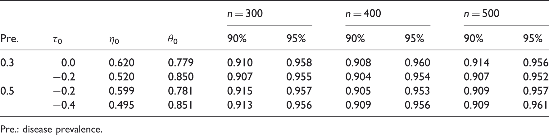
When disease models are misspecified, we will only evaluate confidence regions based on FI, MSI, and SPE methods because the IPW method does not depend on a disease status model. Coverage probabilities (which are from 70% to 80%, not reported here) for FI- and MSI-based confidence regions are much smaller than nominal levels, and the results for SPE-based methods are displayed in Table 2. Table 2 shows that the proposed SPE-based jackknife EL confidence regions work well with moderate sample size cases (

n \geq 300

) when a misspecification of the disease model is present.

Table 2.

Misspecified disease models: Coverage probabilities of SPE-based joint empirical likelihood confidence regions with nominal confidence levels 90% and 95% in the presence of verification bias.

Pre.	τ ₀	η ₀	θ ₀	n = 300		n = 400		n = 500
Pre.	τ ₀	η ₀	θ ₀	90%	95%	90%	95%	90%	95%
0.3	0.0	0.620	0.779	0.910	0.958	0.908	0.960	0.914	0.956
0.3	−0.2	0.520	0.850	0.907	0.955	0.904	0.954	0.907	0.952
0.5	−0.2	0.599	0.781	0.915	0.957	0.905	0.953	0.909	0.957
0.5	−0.4	0.495	0.851	0.913	0.956	0.909	0.956	0.909	0.961

Pre.: disease prevalence.

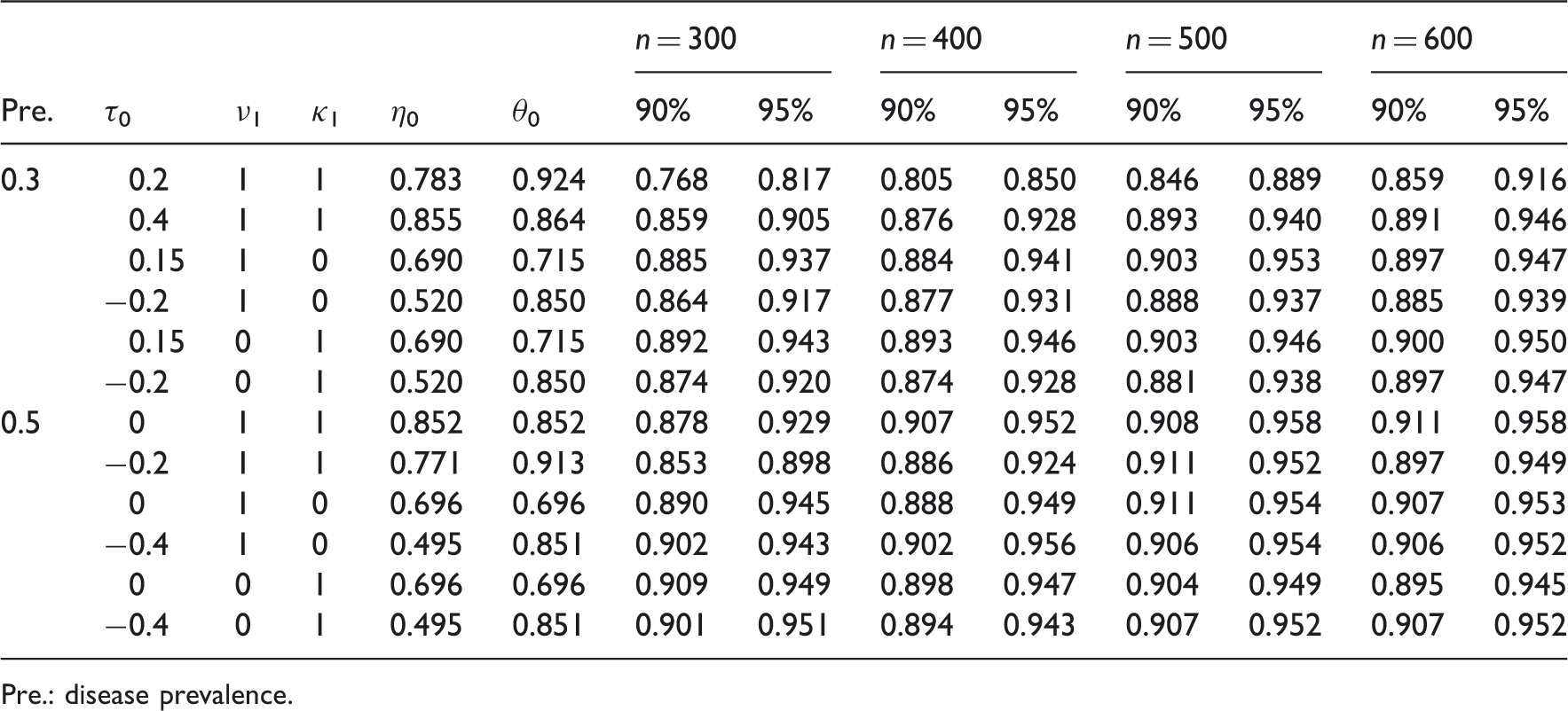
When verification models are misspecified, only confidence regions based on IPW and SPE methods are evaluated, because the FI and MSI methods do not depend on a verification status model. Similarly, coverage probabilities for IPW region are not good (not reported here), and only results from SPE-based method are presented. Table 3 indicates that SPE-based jackknife EL confidence regions work well with moderate sample size cases (

n \geq 300

) for most cases when a misspecification of the verification model is present. In the first case where disease prevalence is 0.3,

ν 1 = κ 1 = 1

, and the cut-off level is selected to generate much higher sensitivity than specificity, resulting joint confidence regions undercover true values. However, from simulation results, it is clear that their performance improves as the sample size increases from 300 to 600. One reasonable explanation for such phenomena is again due to the asymptotic independence of jackknife pseudo samples. In order to get better results, we recommend the proposed methods in Refs. [11] and [12] based on weighted chi-square distributions, which are shown to perform well in all cases for moderate sample sizes

n \geq 300

Table 3.

Misspecified verification models: Coverage probabilities of SPE-based joint empirical likelihood confidence regions with nominal confidence levels 90% and 95% in the presence of verification bias.

Pre.	τ ₀	ν ₁	κ ₁	η ₀	θ ₀	n = 300		n = 400		n = 500		n = 600
Pre.	τ ₀	ν ₁	κ ₁	η ₀	θ ₀	90%	95%	90%	95%	90%	95%	90%	95%
0.3	0.2	1	1	0.783	0.924	0.768	0.817	0.805	0.850	0.846	0.889	0.859	0.916
	0.4	1	1	0.855	0.864	0.859	0.905	0.876	0.928	0.893	0.940	0.891	0.946
	0.15	1	0	0.690	0.715	0.885	0.937	0.884	0.941	0.903	0.953	0.897	0.947
	−0.2	1	0	0.520	0.850	0.864	0.917	0.877	0.931	0.888	0.937	0.885	0.939
	0.15	0	1	0.690	0.715	0.892	0.943	0.893	0.946	0.903	0.946	0.900	0.950
	−0.2	0	1	0.520	0.850	0.874	0.920	0.874	0.928	0.881	0.938	0.897	0.947
0.5	0	1	1	0.852	0.852	0.878	0.929	0.907	0.952	0.908	0.958	0.911	0.958
	−0.2	1	1	0.771	0.913	0.853	0.898	0.886	0.924	0.911	0.952	0.897	0.949
	0	1	0	0.696	0.696	0.890	0.945	0.888	0.949	0.911	0.954	0.907	0.953
	−0.4	1	0	0.495	0.851	0.902	0.943	0.902	0.956	0.906	0.954	0.906	0.952
	0	0	1	0.696	0.696	0.909	0.949	0.898	0.947	0.904	0.949	0.895	0.945
	−0.4	0	1	0.495	0.851	0.901	0.951	0.894	0.943	0.907	0.952	0.907	0.952

Pre.: disease prevalence.

These observations confirm that the SPE-based jackknife EL method is “doubly robust.” As mentioned in Refs. [11] and [12], SPE-based normal approximation regions could perform well in some settings, but results are not stable.

4 Study of neonatal hearing screening data

We apply the proposed various jackknife confidence regions in the presence of verification bias to a neonatal hearing screening data set. This data set is provided by Alonzo and Pepe.⁵ In their paper, they proposed several bias-corrected estimators of true and false positive rates, constructed ROC curves for the Neonatal Hearing screening test, and then estimated areas under those ROC curves.

Undetected hearing loss in infants is of great concern because it results in serious problems with speech, and social and emotional development. Thus, early diagnosis of such conditions is important. The Identification of Neonatal Hearing Impairment (INHI) is a study that aims for assessing the accuracy of two passive electronic devices, the Distortion Product Otoacoustic Emissions (DPOAE) test and the Transient Evoked Otoacoustic Emissions (TEOAE) test. These two tests can be administered soon after birth²⁶ compared with the gold standard test for determining neonatal hearing loss, the Visual Reinforcement Audiometry (VRA) test, which cannot be administered until infants are eight to 12 months old. Therefore, the evaluation of these two screening tests is necessary for the earliest possible diagnosis.

The subset of the INHI data used in this paper was generated by Alonzo and Pepe,⁵ following a two-phase design. In the first phase, DPOAE and TEOAE test results are available for all infants. In the second phase, all infants with DPOAE test results greater than the 80-th quantile of the distribution of DPOAE test results for at least one ear are sent to be verified, and remaining infants are verified with probability 0.4. The subset includes TEOAE and DPOAE test results on 5101 ears, corresponding to 2763 infants. Also, verification statuses V_i’s and VRA results, D_i’s, for 1571 verified infants are available. We follow the same argument in Ref. [5] to let $T \equiv$ DPOAE and $A \equiv$ TEOAE. Both logistic and probit regressions are used to fit $P (D = 1 | T, A)$ to obtain $\overset{\land}{ρ} i$ ’s, and the difference is small. Then, we use a probit regression in the final model. We use 2763 observations, one ear from each infant, in our real case study because the decision to verify by VRA only depends on the ear with larger DPOAE screening test values. For infants with DPOAE test results greater than the 80-th quantile of DPOAE results, the verification proportion $π i = 1$ ; for infants with DPOAE test results below the threshold, $π i = 0.394$ . With this specific large data set, we do not repeatedly estimate ${\overset{\land}{π} j, - i} j = 1, j \neq i n$ for each i required by the jackknife technique. Instead, the counterparts based on the whole sample are used to simplify the calculation.

In order to select a reasonable cut-off point that generates both required sensitivity and specificity of the DPOAE test, we take the idea in Ref. [10] and follow the procedure in Refs. [11] and [12]. First, proper joint confidence regions for the pair of (sensitivity, cut-off level) at a fixed specificity value and the pair of (specificity, cut-off level) at a fixed sensitivity value are constructed to investigate the relationship among sensitivity, specificity, and cut-off level. In order to fix a specificity and a sensitivity, we look at the ROC curves provided in Ref. [5]. From those curves, the DPOAE test performed mediocrely. Therefore, based on the consideration of balanced sensitivity and specificity, we fix both specificity and sensitivity at 0.6. Of course other choices can be made accordingly. With jackknife technique, joint EL confidence regions can be directly constructed by applying Theorem 1. Contour plots are employed to show confidence regions. $l J (θ, 0.6, τ)$ and $l J (0.6, η, τ)$ are evaluated at fine grids of (θ, τ) and (η, τ), and contours are connected according to $(1 - α)$ th quantile of chi-squared distribution with 2 degrees of freedom. Because the true verification model is available, jackknife EL confidence regions based on the IPW method are used as references. Additionally, results from MSI-based jackknife EL with logistic regression assumption of $P (D = 1 | T, A)$ are presented here to make further comparison.

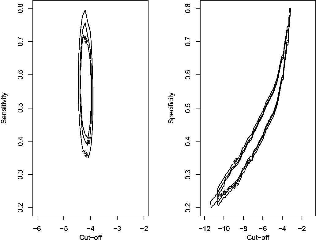
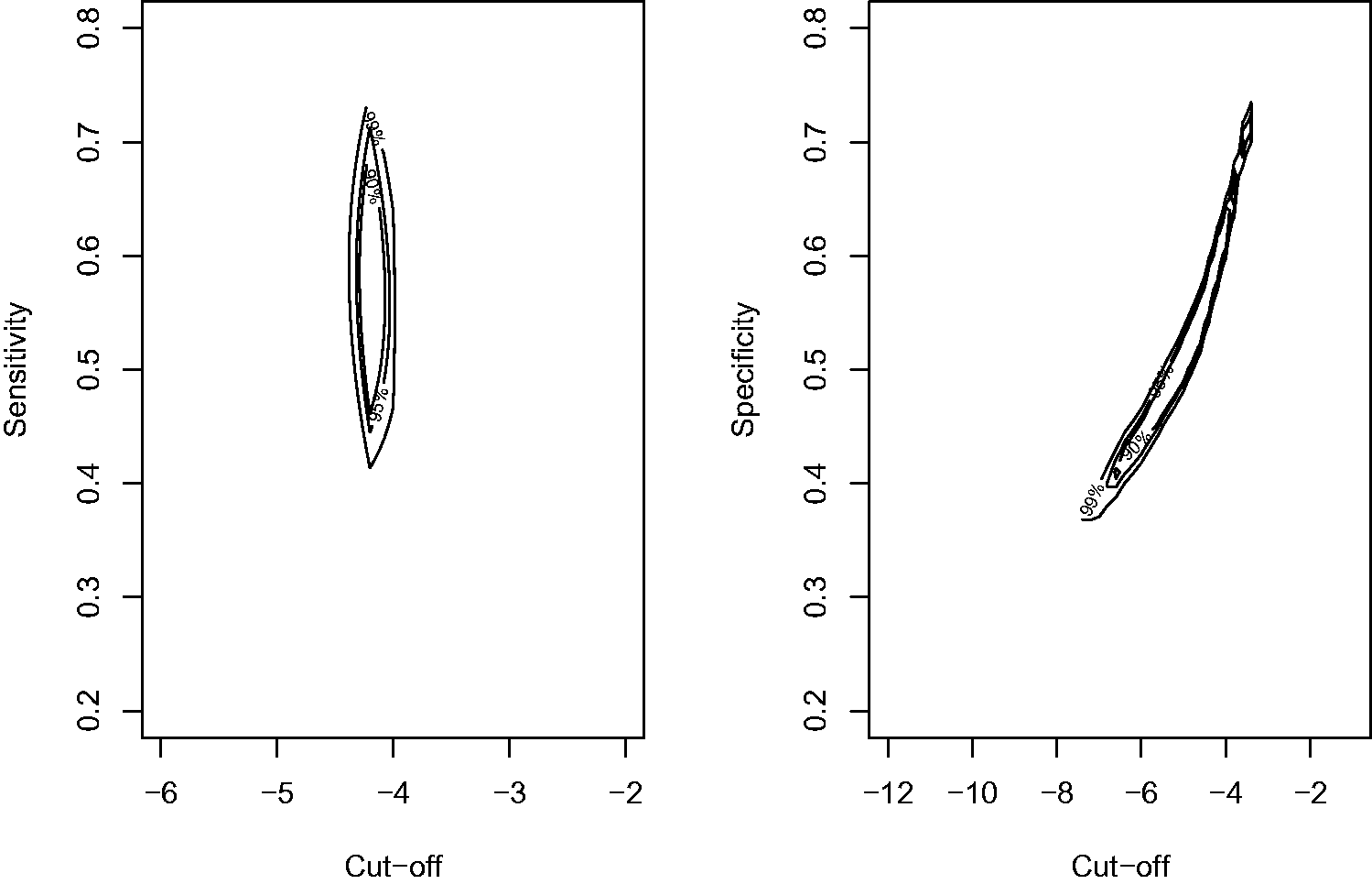
The left panel in Figure 1 shows the contour curves of $l_{IPW}^{J} (θ, 0.6, τ)$ , offering confidence regions for the pair (sensitivity, cut-off level) at nominal confidence levels 90%, 95%, and 99%. The plot indicates that, only a narrow range around 4 of the cut-off level is compatible with the target specificity level of 0.6. The right panel in Figure 1 shows contour curves of $l_{IPW}^{J} (0.6, η, τ)$ , offering confidence regions for the pair (specificity, cut-off level) at nominal levels 90%, 95%, and 99%. This plot shows that, a variety of pairs of values for (η, τ) are compatible with the target sensitivity level of 0.6 in a narrow strip manner. Similarly, we have Figure 2 for $l_{MSI}^{J} (θ, 0.6, τ)$ and $l_{MSI}^{J} (0.6, η, τ)$ . Although, both confidence regions have similar shapes at nominal levels 90% and 95%, MSI-based confidence regions for the pair of specificity and cut-off level have narrower ranges for the cut-off level. Therefore, MSI-based joint confidence regions under logistic regression assumptions for D seems to be optimistic.

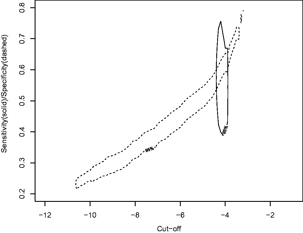
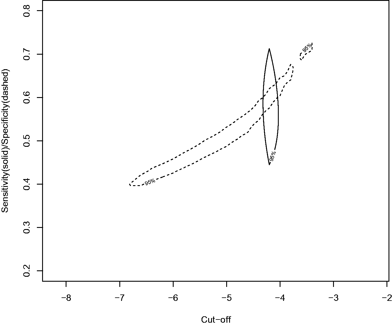
Joint confidence regions offer us a good chance to select reasonable cut-off levels compatible with both required specificity and sensitivity, 0.6 in this study, by plotting two regions in the same graph. Figure 3 shows both 95% IPW-based jackknife joint confidence region for the pair of (sensitivity, cut-off level) at the fixed specificity level of 0.6 and the 95% confidence region for the pair of (specificity, cut-off level) at the fixed sensitivity level of 0.6. Figure 4 shows similar regions from MSI-based jackknife joint confidence regions. The overlapping parts in the two graphs indicate a narrow interval of around −4 as a cut-off level. Therefore, we select −4 as a reasonable value for the cut-off level. Additionally, SPE method-based bias-corrected estimators of sensitivity and specificity in Ref. [5] are applied to evaluate the Youden Index, which suggests −1 as an optimal cut-off level, and the corresponding sensitivity and specificity are 0.381 and 0.869. It seems this cut-off point may not be a good choice because the resulting sensitivity is too small. Instead, cut-off level at −4 provides sensitivity 0.624 and specificity 0.548.

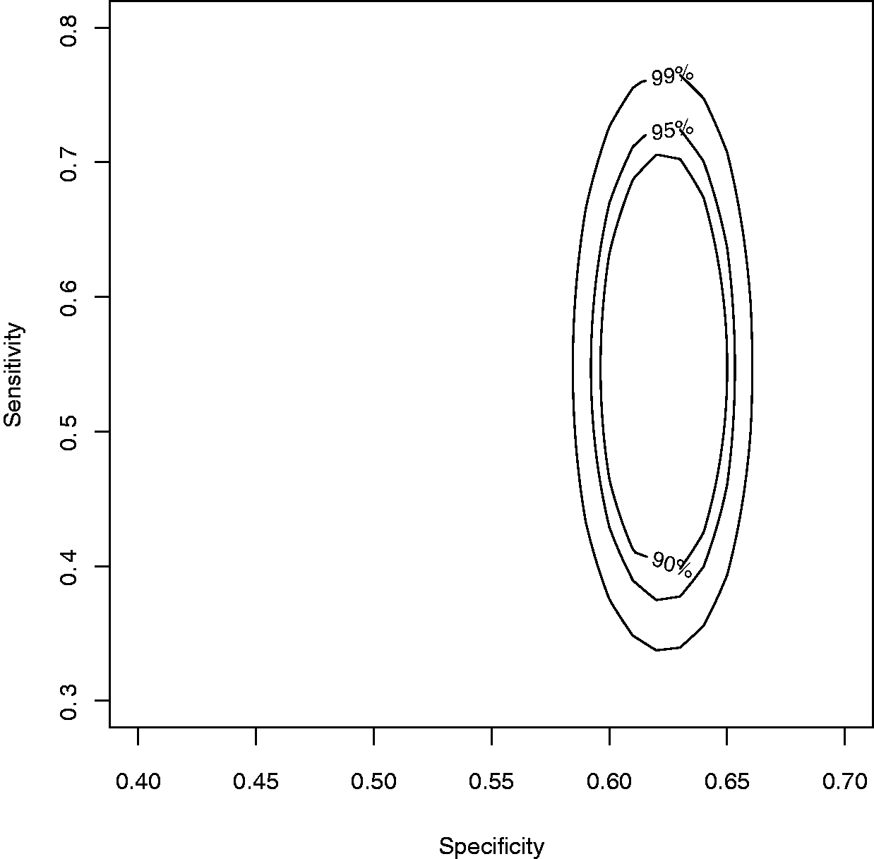
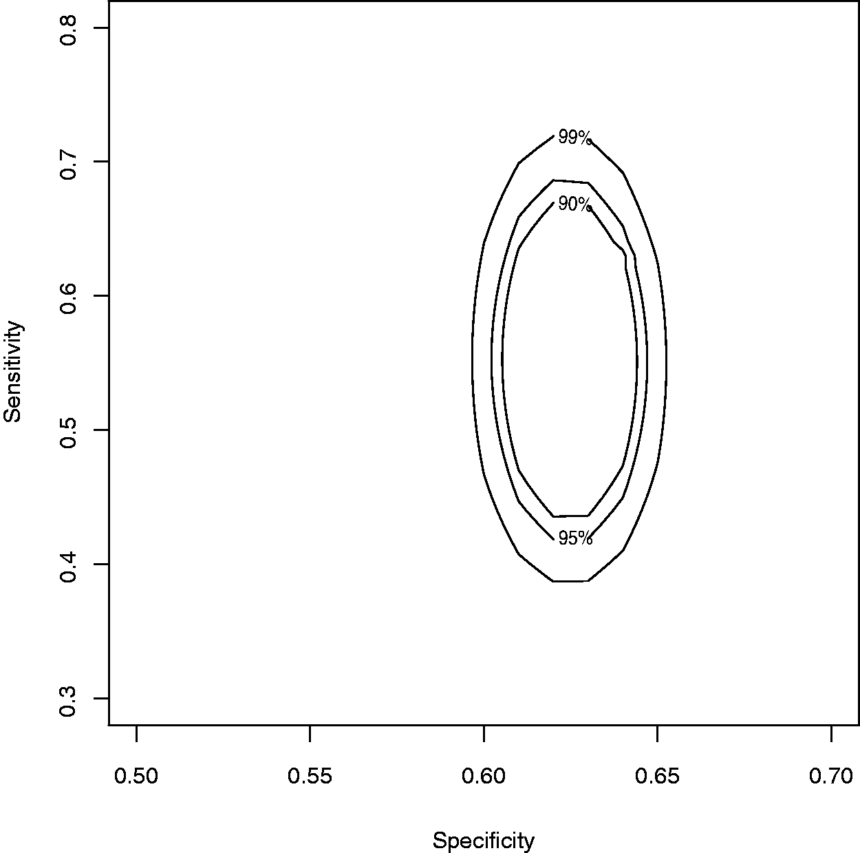
Given the cut-off level, joint confidence regions of the specificity and sensitivity can be obtained. Figures 5 and 6 show contour curves of $l_{IPW}^{J} (θ, η, - 4)$ and $l_{MSI}^{J} (θ, η, - 4)$ , respectively, indicating 95% joint jackknife confidence regions for the pair of (specificity, sensitivity) with the cut-off level fixed at −4. With the cut-off level fixed at −4, in Figure 5 for the IPW-based confidence region, the specificity ranges from 0.58 to 0.67, and the sensitivity ranges from 0.35 to 0.75; in Figure 6, the MSI-based method provides a smaller confidence region, i.e., the specificity ranges from 0.60 to 0.65, and the sensitivity ranges from 0.40 to 0.73. Compared with elliptical confidence regions in Ref. [5], ours have a data driven shape, close to ellipse due to a large sample size.

5 Discussion

In this paper, with the jackknife technique, we successfully reduce the computation burden in applying bias-corrected confidence regions of cut-off and sensitivity; cut-off and specificity; and specificity and sensitivity, proposed in Refs. [11] and [12]. The reason is jackknife EL ratio statistics enjoy standard chi-squared distributions asymptotically.

As suggested by one referee, the MAR assumption is still strong and hard to justify. It is demanding to relax the MAR assumption used here to the MNAR assumption, resulting in the non-ignorable verification bias. There is substantial literature dealing with the non-ignorable verification bias.^25,27–29 The method developed here can potentially be applied to the non-ignorable missing mechanism, because the non-ignorable verification mechanism can be modeled through a non-ignorable parameter.²⁸ Our future research will consider non-ignorable verification bias.

A reasonable cut-off level, which generates required sensitivity and specificity, can be identified from joint confidence regions. This visual method is easy to apply, yet somehow subjective. Additionally, the proposed methods do not take the variation and correlation introduced by the data-dependent estimation of the cut-off into account. Bantis et al.³⁰ provided a good insight on this issue. A further research topic will deal with selecting an optimal cut-off level and take its variation into account.

Footnotes

Declaration of conflicting interests

The author(s) declared no potential conflicts of interest with respect to the research, authorship, and/or publication of this article.

Funding

The author(s) received no financial support for the research, authorship, and/or publication of this article.

References

Begg

Greenes

. Assessment of diagnostic tests when disease is subject to selection bias. Biometrics 1983; 39: 207–216.

Ransohoff

Feinstein

. Problems of spectrum and bias in evaluating the efficacy of diagnostic tests. N Engl J Med 1978; 299: 926–930.

Rubin

. Inferences and missing data. Biometrika 1976; 63: 581–590.

Little

RJA

Rubin

. Statistical analysis with missing data, 2nd edn. New York: John Wiley & Sons, 2002.

Alonzo

Pepe

. Assessing accuracy of a continuous screening test in the presence of verification bias. Appl Stat 2005; 54: 173–190.

Owen

. Empirical likelihood ratio confidence intervals for single functional. Biometrika 1998; 75: 237–249.

Owen

. Empirical likelihood ratio confidence regions. Ann Stat 1990; 18: 90–120.

Owen

. Empirical likelihood, New York: Chapman & Hall/CRC, 2001.

Chen

Van Keilegom

. A review on empirical likelihood methods for regressions (with discussions). Test 2009; 3: 415–447.

10.

Adimari

Chiogna

. Simple nonparametric confidence regions for the evaluation of continuous-scale diagnostic tests. Int J Biostat 2010; 6: Article 24–Article 24.

11.

Wang BH. Statistical evaluation of continuous-scale diagnostic tests with missing data. Mathematics Dissertations, Georgia State University, Atlanta, USA, 2012. Paper 8, http://digitalarchive.gsu.edu/math_diss/8/ (2012, accessed 20 November 2013).

12.

Wang

Qin

. Empirical likelihood confidence regions for the evaluation of continuous-scale diagnostic test in the presence of verification bias. Can J Stat 2013; 41: 398–420.

13.

Jing

Yuan

Zhou

. Jackknife empirical likelihood. J Am Stat Assoc 2009; 104: 1224–1232.

14.

Peng

. Reduce computation in profile empirical likelihood method. Can J Stat 2011; 39: 370–384.

15.

Peng

. Approximate jackknife empirical likelihood method for estimating equations. Can J Stat 2012; 40: 110–123.

16.

Adimari

Chiogna

. Jackknife empirical likelihood based confidence intervals for partial areas under ROC curves. Stat Sinica 2012; 22: 1457–1477.

17.

Qin

Lawless

. Empirical likelihood and general estimating equations. Annu Stat 1994; 22: 300–325.

18.

Tukey

. Bias and confidence in not-quite large samples. Annu Stat 1958; 29: 614–614.

19.

Faraggi

. Adjusting receiver operating curves and related indices for covariates. The Statistician 2003; 52: 179–192.

20.

Schisterman

Faraggi

Reiser

. Youden index and the optimal threshold for markers with mass at zero. Stat Med 2008; 27: C297–C315.

21.

Molanes-López

Letón

. Inference of the Youden index and associated threshold using empirical likelihood for quantiles. Stat Med 2011; 30: 2467C–2480C.

22.

Lai

C-Y

Tian

Schisterman

. Exact confidence interval estimation for the Youden index and its corresponding optimal cut-point. Comput Stat Data Anal 2012; 56: 1103–1114.

23.

Gao

Hui

Hall

. Estimating disease prevalence from two-phase surveys with non-response at the second phase. Stat Med 2000; 19: 2101–2114.

24.

Alonzo

Pepe

Lumley

. Estimating disease prevalence in two-phase studies. Biostatistics 2003; 4: 313–326.

25.

Rotnitzky

Faraggi

Schisterman

. Doubly robust estimation of the area under the receiver-operating characteristic curve in the presence of verification bias. J Am Stat Assoc 2006; 101: 1276–1288.

26.

Norton

Gorga

Widen

. Identification of neonatal hearing impairment: a multicenter investigation. Ear Hear 2000; 21: 348–356.

27.

Fluss

Reiser

Faraggi

. Estimation of the ROC curve under verification bias. Biom J 2009; 51: 475–490.

28.

Liu

Zhou

. A model for adjusting for nonignorable verification bias in estimation of ROC curve and its area with likelihood-based approach. Biometrics 2010; 66: 1119–1128.

29.

Fluss

Reiser

Faraggi

. Adjusting ROC curves for covariates in the presence of verification bias. J Stat Plann Inference 2012; 142: 1–11.

30.

Bantis

Nakas

Reiser

. Construction of confidence regions in the ROC space after the estimation of the optimal Youden index-based cut-off point. Biometrics. Epub ahead of print 21 November 2013. DOI: 10.1111/biom.12107.