Empirical likelihood inference in randomized clinical trials

Abstract

In individually randomized controlled trials, in addition to the primary outcome, information is often available on a number of covariates prior to randomization. This information is frequently utilized to undertake adjustment for baseline characteristics in order to increase precision of the estimation of average treatment effects; such adjustment is usually performed via covariate adjustment in outcome regression models. Although the use of covariate adjustment is widely seen as desirable for making treatment effect estimates more precise and the corresponding hypothesis tests more powerful, there are considerable concerns that objective inference in randomized clinical trials can potentially be compromised. In this paper, we study an empirical likelihood approach to covariate adjustment and propose two unbiased estimating functions that automatically decouple evaluation of average treatment effects from regression modeling of covariate–outcome relationships. The resulting empirical likelihood estimator of the average treatment effect is as efficient as the existing efficient adjusted estimators¹ when separate treatment-specific working regression models are correctly specified, yet are at least as efficient as the existing efficient adjusted estimators¹ for any given treatment-specific working regression models whether or not they coincide with the true treatment-specific covariate–outcome relationships. We present a simulation study to compare the finite sample performance of various methods along with some results on analysis of a data set from an HIV clinical trial. The simulation results indicate that the proposed empirical likelihood approach is more efficient and powerful than its competitors when the working covariate–outcome relationships by treatment status are misspecified.

Keywords

Average treatment effect clinical trial covariate adjustment efficiency empirical likelihood influence function randomization regression unbiased estimating function

1 Introduction

The invention and use of randomization in the design of an experiment was one of the early major advances in statistical inference. Randomized clinical trials are routinely performed with the goal of assessing the effect of a treatment versus a control. A common measure or estimand for evaluating the treatment effect in the primary analysis is the average treatment effect: the difference in mean outcome between the treatment and control. Because of the randomization, one attractive feature of random assignment of treatments is that it naturally leads to an unbiased estimator of the average treatment effect, which is the difference in the average outcomes between those assigned to treatment and those assigned to control. Thus, randomization is considered by many clinicians and (bio)statisticians to be the “gold standard” of clinical study design.

In many randomized clinical trials, extensive covariate data are collected at baseline for each subject prior to a treatment being assigned, such as pretreatment outcome data, data on prior medical history, data on medications and lab results, demographic data, and so on. Although a key characteristic of these covariates is that they are known a priori to be unaffected by the treatment assignment, the covariates can be highly predictive of the outcomes in many scenarios. As a result, the information available in these covariates can be desirable in that it can be used to make estimates more precise and hypothesis tests more powerful by explaining some of the variation in outcomes; this is the so-called covariate adjustment. The aforementioned unbiased estimator of the average treatment effect ignores this covariate information and may therefore lack efficiency and power compared to analyses that involve covariate adjustment.

There is a vast body of literature dealing with covariate adjustment.^1–9 While covariate adjustment may increase precision and improve power to detect a treatment effect, considerable debate exists as to whether such adjustment is appropriate.^10–13 A major concern of covariate adjustment is the potential compromise of objective inference, resulting from the post hoc selection of covariates and going on a fishing expedition to seek models that yield the most significant treatment effect estimate. Another issue is the potential for biased estimation of treatment effects due to possible misspecification of the associations between the outcome and covariates. Such concerns stem by nature from the standpoint that randomization is necessary for objective inference and that covariate adjustment may inadvertently prompt an accentuation of estimated treatment effects under randomized studies.

To address the aforementioned concerns, there are a number of recent attempts at adjusting covariates objectively in randomized trials. Among others, Tsiatis et al.¹ have proposed a systematic approach to the covariate adjustment problem from a semiparametric theory perspective. Their approach allows for a principled and flexible covariate-adjusted analysis that utilizes regression analysis to exploit covariate–outcome relationships by positing two separate working regression models for the data from the treatment and control arms. In two recent related works, Shen et al.¹⁴ and Williamson et al.¹⁵ have proposed two two-stage estimation procedures for covariate adjustment based on the inverse probability weighting (IPW) method of Horvitz and Thompson¹⁶; one key feature of their procedures is its flexibility of allowing data analysts to adjust covariates before seeing the outcome data.

In this paper, we propose an alternative approach to covariate adjustment in the estimation of average treatment effects. Working from the viewpoint that decouples evaluation of the average treatment effect from regression modeling the outcome and covariate data, we consider two unbiased estimating functions. The first one is associated with the standard “unadjusted” treated-minus-control difference in sample means, which does not take covariates into account and thus depends only on the outcome and treatment assignment indicator. The second one is motivated by the desire for exploitation of covariate–outcome relationships to improve on the unadjusted estimator. For the second estimating function, we focus only on the data on (pretreatment) covariate values and treatment assignment, without having to see the outcome data. As a result, these two estimating functions automatically separate modeling of covariate–outcome relationships from estimation of the average treatment effect, thus providing another attempt at making objective covariate adjustment in randomized clinical trials.

The aforementioned two unbiased estimating functions form the basis for making objective inference on the average treatment effect in randomized studies. Since there are more estimating equations than the parameter of interest, we employ the empirical likelihood method to combine these estimating functions, which leads naturally to an empirical-likelihood-based estimator of the average treatment effect. The proposed empirical likelihood estimator objectively adjusts baseline covariates and simultaneously exploits covariate information to enhance desired efficiency gains. There are three attractive features of the proposed estimator: (a) it is at least as efficient as the unadjusted estimator, i.e. the difference in average observed outcomes by treatment status, (b) it is as efficient as the adjusted estimator proposed by Tsiatis et al.¹ when separate treatment-specific working regression models are correctly specified, and (c) it is at least as efficient as the adjusted estimator of Tsiatis et al.¹ for any given treatment-specific working regression models whether or not they coincide with the true treatment-specific covariate–outcome relationships. Additionally, we demonstrate that when the working covariate–outcome relationships by treatment status are misspecified, (1) the proposed empirical-likelihood-based estimator is more efficient than its competitors theoretically and via simulation, and (2) the proposed empirical-likelihood-based Wald test statistic is more powerful than other existing Wald test statistics via simulation.

As a nonparametric method, empirical likelihood was introduced by Owen^17–21 for constructing confidence intervals or regions for the mean and other parameters. In the context of analyzing data from pretest–posttest randomized trials, Huang et al.²² have proposed an empirical likelihood-based approach to estimation of the average treatment effect without and with missing data on the posttest response; this approach incorporates the common baseline covariate information to improve efficiency.

In Section 2, we provide some notations and a brief review of the existing methodology in covariate adjustment. In Section 3, we propose two unbiased estimating functions and study maximum empirical likelihood estimation of the average treatment effect. In Section 4, we study efficiency comparison between the proposed and existing estimators. In Section 5, the proposed methodology is illustrated using a data set from the AIDS Clinical Trials Group (ACTG) protocol: 175.²³ Simulation results are presented in Section 6 and concluding remarks are given in Section 7. Theorems and their proofs of the main theoretical results are delegated to the supplementary Web Appendix.

2 Notation and review

Consider a clinical trial where n subjects are randomly sampled from a population of interest and are randomized to an experimental treatment or to a standard or control treatment. Let the treatment assignment indicator D take on value 1 if a subject received the experimental treatment, and value 0 if a subject received the control treatment. Furthermore, let $π = P (D = 1)$ be the randomization probability that a subject is assigned to receive the experimental treatment, so that $1 - π$ is the randomization probability that a subject is assigned to receive the control treatment. We are interested in the effect of the treatment D on a continuous or discrete outcome Y. Often, the population of interest is characterized by a $p \times 1$ vector of pretreatment or baseline covariates, X. Randomization implies that D and X are statistically independent. The observed data from the clinical trial are the independent and identically distributed sample $(Y_{i}, D_{i}, X_{i})$ for $i = 1, \dots, n .$ Let $n_{1} = \sum_{i = 1}^{n} D_{i}$ denote the numbers of subjects in the treatment arm, so that $n_{0} = n - n_{1}$ is the numbers of subjects in the control arm.

The average treatment effect is defined as the difference of the pair of the treatment-specific mean outcomes, averaged over the entire population

θ = E (Y | D = 1) - E (Y | D = 0)

(1)

A widely used estimator of θ is the simple difference

{\hat{θ}}_{s} = {\bar{Y}}_{(1)} - {\bar{Y}}_{(0)}

in sample means for treated and controls without adjustment for the covariate vector X, where

{\bar{Y}}_{(1)} = n_{1}^{- 1} \sum_{i = 1}^{n} D_{i} Y_{i}

and

{\bar{Y}}_{(0)} = n_{0}^{- 1} \sum_{i = 1}^{n} (1 - D_{i}) Y_{i}

are the averages of the observed outcomes in the treatment and control groups, respectively. Since

E (Y | D) = E (Y | D = 0) + θ D,

the estimator

{\hat{θ}}_{s}

is shown to be the least squares estimator of the coefficient α₁ for the treatment indicator by specifying a simple linear regression model for the observed outcome as

Y_{i} = α_{0} + α_{1} D_{i} + ɛ_{i}

for

i = 1, \dots, n,

where

ɛ_{i}

is a random error with mean

E (ɛ_{i}) = 0

. This well-known phenomenon motivates a common way of estimating θ based on regression methods by specifying a linear regression function for the observed outcome as a function of a set of predictor variables, which includes both the treatment assignment indicator and additional pretreatment covariates (and possibly their interactions if the association between the outcome and covariates varies by treatment status); this gives rise to popular covariate adjustment in the estimation of the average treatment effect θ in randomized clinical trials. Two widely known regression estimators of θ are the least-squares estimated coefficients

{\hat{γ}}_{1}

and

{\hat{δ}}_{1}

of the D_i from the analysis of covariance (ANCOVA) model without interactions, i.e.

Y_{i} = γ_{0} + γ_{1} D_{i} + γ_{2}^{τ} X_{i} + ɛ_{i}

, and from the centered ANCOVA model with interactions, i.e.

Y_{i} - \bar{Y} = δ_{0} + δ_{1} (D_{i} - \bar{D}) + δ_{2}^{τ} (X_{i} - \bar{X}) + δ_{3}^{τ} (D_{i} - \bar{D}) (X_{i} - \bar{X}) + ɛ_{i}

, where

\bar{Y} = n^{- 1} \sum_{i = 1}^{n} Y_{i},

\bar{D} = n^{- 1} \sum_{i = 1}^{n} D_{i},

and

\bar{X} = n^{- 1} \sum_{i = 1}^{n} X_{i} .

Write

{\hat{θ}}_{reg 1} = {\hat{γ}}_{1}

and

{\hat{θ}}_{reg 2} = {\hat{δ}}_{1} .

Under standard regularity conditions, the standard unadjusted estimator

{\hat{θ}}_{s}

and popular adjusted estimators

{\hat{θ}}_{reg 1}

and

{\hat{θ}}_{reg 2}

have been shown to be consistent and asymptotically normal for

θ .

The estimators ${\hat{θ}}_{reg 1}$ and ${\hat{θ}}_{reg 2}$ may be regarded as one-stage estimators of θ in the sense that they are based on models for the regression of Y on both D and X at the same time, thus causing concerns of subjectivity by inevitably linking the effect of treatment to that of the covariates. To objectively incorporate covariate effects into the evaluation of the treatment effect, Tsiatis et al.¹ have proposed a principled approach to covariate adjustment from the perspective of semiparametric theory, which allows to model covariate effects by treatment status. To describe their principled adjustment methodology, let $m_{k} (X, β_{(k)})$ denote a working regression model for the treatment-specific conditional expectation $E (Y | D = k, X),$ where $β_{(k)}$ is a $p_{k} \times 1$ vector parameter for $k = 0, 1 .$ For the postulated model $m_{k} (X, β_{(k)}),$ let ${\hat{β}}_{(k)}$ be a consistent estimator of $β_{(k)}$ based on the treatment-specific data ${(Y_{i}, D_{i} = k, X_{i}), i = 1, \dots, n}$ for $k = 0, 1 .$ Tsiatis et al.¹ have proposed to estimate θ by

{\hat{θ}}_{tdzl} = {\bar{Y}}_{(1)} - {\bar{Y}}_{(0)} - \sum_{i = 1}^{n} (D_{i} - \bar{D}) {\frac{1}{n_{0}} m_{0} (X_{i}, {\hat{β}}_{(0)}) + \frac{1}{n_{1}} m_{1} (X_{i}, {\hat{β}}_{(1)})}

(2)

and have shown that the estimator

{\hat{θ}}_{tdzl}

is consistent and asymptotically normal for any posited models

m_{0} (X, β_{(0)})

and

m_{1} (X, β_{(1)}),

and is semiparametrically efficient if both models are identical to the true covariate–outcome relationships by treatment status, i.e.

m_{0} (X, β_{00}) = E (Y | D = 0, X)

and

m_{1} (X, β_{10}) = E (Y | D = 1, X),

where β₀₀ and β₁₀ denote the true values of

β_{(0)}

and

β_{(1)} .

In the pretest–posttest setting, Huang et al.²² have proposed a semiparametric procedure for the estimation of θ using the method of empirical likelihood. Their approach is to first estimate $E (Y | D = 1)$ and $E (Y | D = 0)$ separately, say, by $\hat{E} (Y | D = 1)$ and $\hat{E} (Y | D = 0)$ using two possibly different sets of constraints that incorporate baseline covariates for adjustment and efficiency gains, and then estimate θ by taking their difference to obtain ${\hat{θ}}_{hqf} = \hat{E} (Y | D = 1) - \hat{E} (Y | D = 0) .$ The large sample distribution of ${\hat{θ}}_{hqf}$ follows from the large sample properties of $\hat{E} (Y | D = 1)$ and $\hat{E} (Y | D = 0)$ .

Recently, Shen et al.¹⁴ have applied the IPW method to covariate adjustment in randomized studies. Let $π (x, ξ)$ be a correctly specified parametric model for the propensity score $P (D = 1 | X = x) = P (D = 1)$ that encompasses the true treatment assignment probability $π_{0} = P (D = 1),$ i.e. $π (x, ξ_{0}) = π_{0}$ for all x, where ξ₀ is the truth of $ξ .$ Then the IPW estimator of θ proposed by Shen et al.¹⁴ is given by

{\hat{θ}}_{sll} = \frac{1}{n} \sum_{i = 1}^{n} {\frac{D_{i} Y_{i}}{π (X_{i}; \hat{ξ})} - \frac{(1 - D_{i}) Y_{i}}{1 - π (X_{i}; \hat{ξ})}}

(3)

where

\hat{ξ}

is the maximum likelihood estimator of

ξ .

For the logistic propensity score,

{\hat{θ}}_{sll}

is asymptotically equivalent to

{\hat{θ}}_{reg 2}

and hence is at least as efficient as

{\hat{θ}}_{s} .

Similarly, Williamson et al.¹⁵ have proposed an inverse probability-of-treatment weighting estimator of θ with weights

D_{i} {π (X_{i}; \hat{ξ})}^{- 1}

and

(1 - D_{i}) {1 - π (X_{i}; \hat{ξ})}^{- 1}

replaced by the standardized weights

D_{i} {π (X_{i}; \hat{ξ})}^{- 1} / \sum_{i = 1}^{n} D_{i} {π (X_{i}; \hat{ξ})}^{- 1}

and

(1 - D_{i}) {1 - π (X_{i}; \hat{ξ})}^{- 1} / \sum_{i = 1}^{n} (1 - D_{i}) {1 - π (X_{i}; \hat{ξ})}^{- 1},

respectively.

3 Methodology

We now consider an alternative semiparametric approach to covariate adjustment using the method of empirical likelihood. Let $m (X, β)$ be a $q \times 1$ vector function of X and $β,$ a $p \times 1$ vector parameter. Typically, the components of $m (X, β)$ are treatment-specific working regression functions for $E (Y | D = 0, X)$ and $E (Y | D = 1, X) .$ Since $E {(D - π) m (X, β)} = 0$ by randomization and

θ = E (Y | D = 1) - E (Y | D = 0) = E {\frac{DY}{π} - \frac{(1 - D) Y}{1 - π}}

we are motivated to consider two unbiased estimating functions

g_{1} (D, Y, θ, π) = \frac{DY}{π} - \frac{(1 - D) Y}{1 - π} - θ, g_{2} (D, X, π, β, m) = \frac{D - π}{π (1 - π)} {m (X, β) - m}

(4)

where

m = E {m (X, β)} .

Note that the first estimating function

g_{1} (D, Y, θ, π)

involves data only on outcome and treatment assignment, whereas the second estimating function

g_{2} (D, X, π, β, m)

involves data only on covariates and treatment assignment. Therefore,

g_{1} (D, Y, θ, π)

and

g_{2} (D, X, π, β, m)

automatically separate adjustment for covariate effects from estimation of the treatment effect. Note also that

m (X, β)

is a vector function whose dimension equals 1 or 2 in most cases. If we posit the same working regression model for both

E (Y | D = 0, X)

and

E (Y | D = 1, X),

then the dimension of

m (X, β)

is 1. On the other hand, if we posit different working regression models for

E (Y | D = 0, X)

and

E (Y | D = 1, X),

then the dimension of

m (X, β)

is 2. In addition, if we postulate multiple models from robustness considerations for each treatment-specific conditional expectation

E (Y | D = k, X)

with

k = 0, 1,

then the dimension of

m (X, β)

may be more than 1.

Our focus of attention in this paper is on the estimation of the average treatment effect θ, the parameter of interest. Since the number of estimating functions in equation (4) is at least as large as 2 (depending on the dimension of $m (X, β)$ ), which is greater than the dimension 1 of θ, the question arises as how to combine the two estimating functions in equation (4) to estimate $θ .$ The empirical likelihood method of Owen^17–18 and Qin and Lawless¹⁹ provides an effective way of combining unbiased estimating functions when the number of estimating functions exceeds the number of parameters of interest. Considering the fact that the estimating functions $g_{1} (D, Y, θ, π)$ and $g_{2} (D, X, π, β, m)$ also depend on the nuisance parameters $π,$ $β,$ and m, we study a pseudo-empirical likelihood approach to estimating $θ .$ To this end, let $\hat{β}$ be an estimator of β such that the components of β are estimated using the treatment-specific data ${(Y_{i}, D_{i} = k, X_{i}), i = 1, \dots, n}$ for $k = 0, 1,$ and let $\hat{π} = \bar{D}$ and $\hat{m} = n^{- 1} \sum_{i = 1}^{n} m (X_{i}, \hat{β}) .$ Moreover, write $g (D, Y, X, θ, π, β, m) = (g_{1} (D, Y, θ, π), g_{2}^{τ} (D, X, π, β, m))^{τ} .$ Throughout this paper, let $(θ_{0}, π_{0}, β_{0}, m_{0})$ denote the truth of $(θ, π, β, m),$ so that $m_{0} = E {m (X, β_{0})} .$ Furthermore, let $β^{*}$ represent the probability limit of $\hat{β}$ and $m^{*} = E {m (X, β^{*})} .$ When the components of $m (X, β)$ pertain to working regression models that coincide with the true treatment-specific covariate–outcome relationships, we have $β^{*} = β_{0}$ and $m^{*} = m_{0}$ .

Let $(Y, D, X) \sim F;$ then $E_{F} {g (D, Y, X, θ, π, β, m)} = 0 .$ To implement the pseudo-empirical likelihood estimation of θ, we first estimate $(π, β, m)$ by $(\hat{θ}, \hat{β}, \hat{m}),$ and then maximize the nonparametric likelihood $L_{F} = Π_{i = 1}^{n} p_{i}$ subject to the constraints $\sum_{i = 1}^{n} p_{i} = 1, p_{i} \geq 0$ , $\sum_{i = 1}^{n} p_{i} g (D_{i}, Y_{i}, X_{i}, θ, \hat{π}, \hat{β}, \hat{m})$ $= 0,$ where $p_{i} = dF (Y_{i}, D_{i}, X_{i}),$ $i = 1, \dots, n,$ are nonnegative jump sizes with total mass unity. For fixed θ, an application of the Lagrange multipliers method shows that the maximum value of L_F is attained at ${\hat{p}}_{i} (θ) = n^{- 1} {1 + λ_{n}^{τ} g (D_{i}, Y_{i}, X_{i}, θ, \hat{π}, \hat{β}, \hat{m})}^{- 1},$ where $λ_{n} = λ_{n} (θ)$ is determined by

\frac{1}{n} \sum_{i = 1}^{n} \frac{g (D_{i}, Y_{i}, X_{i}, θ, \hat{π}, \hat{β}, \hat{m})}{1 + λ^{τ} g (D_{i}, Y_{i}, X_{i}, θ, \hat{π}, \hat{β}, \hat{m})} = 0 .

(5)

After profiling the p_i’s, the profile log pseudo-empirical likelihood function of θ is given by

ℓ (θ) = ℓ (θ, λ_{n} (θ)),

where

ℓ (θ, λ) = - \sum_{i = 1}^{n} \log {1 + λ^{τ} g (D_{i}, Y_{i}, X_{i}, θ, \hat{π}, \hat{β}, \hat{m})} - n \log n

(6)

Let

{\hat{θ}}_{el}

denote the maximum pseudo-empirical likelihood (MPEL) estimator of θ, which maximizes

ℓ (θ) .

Theorem 1 summarizes the large sample results of

{\hat{θ}}_{el}

; this theorem and its proof are given in the supplementary Web Appendix.

The asymptotic expansion of ${\hat{θ}}_{el}$ in Theorem 1 provides a revealing insight into the potential efficiency gain by employing the empirical likelihood method for covariate adjustment in randomized trials; we will discuss the efficiency comparison of ${\hat{θ}}_{el}$ with other competitive estimators in Section 4. To make inference for θ, the asymptotic variance $σ_{el}^{2}$ of ${\hat{θ}}_{el}$ can be consistently estimated by

{\hat{σ}}_{el}^{2} = C \sum_{i = 1}^{n} {\hat{p}}_{i} [\frac{D_{i} Y_{i}}{\bar{D}} - \frac{(1 - D_{i}) Y_{i}}{1 - \bar{D}} - \frac{D_{i} - \bar{D}}{\bar{D} (1 - \bar{D})} \hat{η} - {\hat{θ}}_{el} - {\hat{S}}_{12} {\hat{S}}_{22}^{- 1} \frac{D_{i} - \bar{D}}{\bar{D} (1 - \bar{D})} {m (X_{i}, \hat{β}) - \hat{m}}]^{2}

where

{\hat{p}}_{i} = {\hat{p}}_{i} ({\hat{θ}}_{el})

for

i = 1, \dots, n,

C is a small sample “correction factor” described below, and

\begin{array}{l} \hat{η} = \frac{1}{n} \sum_{i = 1}^{n} {\frac{\bar{D}}{1 - \bar{D}} (1 - D_{i}) Y_{i} + \frac{1 - \bar{D}}{\bar{D}} D_{i} Y_{i}}, \\ {\hat{S}}_{12} = \frac{1}{\bar{D} (1 - \bar{D})} \sum_{i = 1}^{n} {\hat{p}}_{i} {\frac{D_{i} Y_{i}}{\bar{D}} - \frac{(1 - D_{i}) Y_{i}}{1 - \bar{D}}} (D_{i} - \bar{D}) {m (X_{i}, \hat{β}) - \hat{m}}^{τ}, \\ {\hat{S}}_{22} = \frac{1}{\bar{D} (1 - \bar{D})} \sum_{i = 1}^{n} {\hat{p}}_{i} {m (X_{i}, \hat{β}) - \hat{m}} {m (X_{i}, \hat{β}) - \hat{m}}^{τ} \end{array}

As in Tsiatis et al.,¹ we take

C = (n - 1) / (n - q - 1)

if we posit the same working regression model

m (X, β)

with q parameters (excluding the intercept) for both

E (Y | D = 0, X)

and

E (Y | D = 1, X),

and take

C = {(n_{0} - q_{0} - 1)^{- 1} + (n_{1} - q_{1} - 1)^{- 1}} / {(n_{0} - 1)^{- 1} + (n_{1} - 1)^{- 1}}

when we posit separate working regression models

m_{k} (X, β_{(k)})

with q_k parameters (exclusive of intercepts) for

E (Y | D = k, X),

k = 0, 1 .

The asymptotic normality of

{\hat{θ}}_{el}

in Theorem 1 implies that a level

1 - α

Wald confidence interval for the average treatment effect θ is given by

{\hat{θ}}_{el} \pm z_{1 - α / 2} {\hat{σ}}_{el} / \sqrt{n},

where

z_{1 - α / 2}

satisfies

P (Z \leq z_{1 - α / 2}) = 1 - α / 2

with

Z \sim N (0, 1) .

To test the null hypothesis that the average treatment effect is zero against the alternative hypothesis that the average treatment effect differs from zero:

H_{0} : θ = 0

versus

H_{0} : θ \neg = 0,

we can employ the Wald test statistic

\sqrt{n} {\hat{θ}}_{el} / {\hat{σ}}_{el}

and reject the null hypothesis

H_{0} : θ = 0

at level α if

\sqrt{n} | {\hat{θ}}_{el} | / {\hat{σ}}_{el} > z_{1 - α / 2} .

We close this section by discussing the optimal choice of $m (X, β),$ which is an arbitrary and user-specified vector function. Since the components of $m (X, β)$ specifies working regression models for the treatment-specific outcome–covariate relationships, there can be many different possible choices for $m (X, β) .$ Theorem 2 in the supplementary Web Appendix identifies the optimal choice of $m (X, β),$ which minimizes the asymptotic variance $σ_{el}^{2}$ of ${\hat{θ}}_{el}$ over all choices of $m (X, β) .$ The proof of Theorem 2 is also given in the supplementary Web Appendix.

4 Efficiency comparison

To compare the proposed MPEL estimator ${\hat{θ}}_{el}$ with other existing estimators, we employ the notion of influence functions. For an exposition on influence functions, see, for example, Tsiatis.²⁴

We first compare ${\hat{θ}}_{el}$ with the standard unadjusted estimator ${\hat{θ}}_{s} = {\bar{Y}}_{(1)} - {\bar{Y}}_{(0)} .$ It can be shown that the influence function of ${\hat{θ}}_{s}$ is identical to

ψ_{s} (D, Y, θ_{0}, π_{0}, η_{0}) = g_{1} (D, Y, θ_{0}, π_{0}) - \frac{D - π_{0}}{π_{0} (1 - π_{0})} η_{0}

Furthermore, according to Theorem 1, the asymptotic expansion of

{\hat{θ}}_{el}

in equation (A.1) of the supplementary Web Appendix implies that the influence function of

{\hat{θ}}_{el}

is equal to

ψ_{el} (D, Y, X, θ_{0}, π_{0}, β^{*}, m^{*}, η_{0}) = ψ_{s} (D, Y, θ_{0}, π_{0}, η_{0}) - S_{12} S_{22}^{- 1} g_{2} (D, X, π_{0}, β^{*}, m^{*})

where S₁₂ and S₂₂ are defined in equation (A.2) of the supplementary Web Appendix. Let

Λ = {A g_{2} (D, X, π_{0}, β_{0}, m_{0}) for all 1 \times q real vectors A}

(7)

denote the linear space spanned by

g_{2} (D, X, π_{0}, β_{0}, m_{0})

and let

Π {g_{1} (D, Y, θ_{0}, π_{0}) | Λ}

represent the projection of

g_{1} (D, Y, θ_{0}, π_{0})

onto the space

Λ .

Since

(D - π_{0}) η_{0} / π_{0} (1 - π_{0})

is orthogonal to the linear space Λ, it can be shown after some algebra that

Π {ψ_{s} (D, Y, θ_{0}, π_{0}, η_{0}) | Λ} = S_{12} S_{22}^{- 1} g_{2} (D, X, π_{0}, β^{*}, m^{*})

This implies that

ψ_{el} (D, Y, X, θ_{0}, π_{0}, β^{*}, m^{*}, η_{0})

is the residual from the projection of

ψ_{s} (D, Y, θ_{0}, π_{0},

η_{0})

onto the space

Λ .

We can now deduce from the theory of influence functions that the asymptotic variance of

{\hat{θ}}_{el}

is less than or equal to that of

{\hat{θ}}_{s}

AVar ({\hat{θ}}_{el}) = E {ψ_{el}^{2} (D, Y, X, θ_{0}, π_{0}, β^{*}, m^{*}, η_{0})} \leq E {ψ_{s}^{2} (D, Y, θ_{0}, π_{0}, η_{0})} = AVar ({\hat{θ}}_{s})

Therefore, ${\hat{θ}}_{el}$ is asymptotically at least as efficient as ${\hat{θ}}_{s}$ for any vector function $m (X, β),$ whether or not the components of $m (X, β)$ correctly identify the true treatment-specific conditional expectations $E (Y | D = 0, X)$ and $E (Y | D = 1, X) .$

Second, we compare ${\hat{θ}}_{el}$ with the regression estimators ${\hat{θ}}_{reg 1}$ and ${\hat{θ}}_{reg 2} .$ According to Tsiatis et al.,¹ the influence functions of ${\hat{θ}}_{reg 1}$ and ${\hat{θ}}_{reg 2}$ are, respectively, given by

\begin{array}{l} ψ_{reg 1} (D, Y, X, θ_{0}, π_{0}, η_{0}) = ψ_{s} (D, Y, θ_{0}, π_{0}, η_{0}) - Σ_{X Y}^{τ} Σ_{X X}^{- 1} \frac{D - π_{0}}{π_{0} (1 - π_{0})} {X - E (X)} \\ ψ_{reg 2} (D, Y, X, θ_{0}, π_{0}, η_{0}) = ψ_{s} (D, Y, θ_{0}, π_{0}, η_{0}) - {π_{0} Σ_{X Y}^{(0)} + (1 - π_{0}) Σ_{X Y}^{(1)}}^{τ} Σ_{X X}^{- 1} \frac{D - π_{0}}{π_{0} (1 - π_{0})} {X - E (X)} \end{array}

where

Σ_{XY} = Cov (X, Y) = (1 - π_{0}) Σ_{XY}^{(0)} + π_{0} Σ_{XY}^{(1)},

Σ_{XX} = Var (X),

and

Σ_{XY}^{(k)} = E [{X - E (X)} {Y - E (Y)} | D = k], k = 0, 1 .

When

π_{0} = 0.5

or when the covariance between the outcome and covariates is the same for both the treatment and control groups, i.e.

Σ_{XY}^{(0)} = Σ_{XY}^{(1)},

it is seen that

{\hat{θ}}_{reg 1}

and

{\hat{θ}}_{reg 2}

possess the same influence function and are thus asymptotically equivalent. If we choose

m (X, β) = X

for all

β,

then it can be shown after some algebra that

S_{12} = \frac{1}{π_{0} (1 - π_{0})} {π_{0} Σ_{XY}^{(0)} + (1 - π_{0}) Σ_{XY}^{(1)}}^{τ}, S_{22} = \frac{1}{π_{0} (1 - π_{0})} Σ_{XX}

In this case, we have

ψ_{el} (D, Y, X, θ_{0}, π_{0}, β^{*}, m^{*}, η_{0}) = ψ_{reg 2} (D, Y, X, θ_{0}, π_{0}, η_{0}),

and hence

{\hat{θ}}_{el}

and

{\hat{θ}}_{reg 2}

are asymptotically equivalent. Also in this case, since the second term in

ψ_{reg 1} (D, Y, X, θ_{0}, π_{0}, η_{0})

belongs to the space Λ in equation (7), we have

AVar ({\hat{θ}}_{el}) = AVar ({\hat{θ}}_{reg 2}) = E {ψ_{reg 2}^{2} (D, Y, X, θ_{0}, π_{0}, η_{0})} \leq E {ψ_{reg 1}^{2} (D, Y, X, θ_{0}, π_{0}, η_{0})} = AVar ({\hat{θ}}_{reg 1})

Therefore, we conclude that when

m (X, β) = X

for all

β,

{\hat{θ}}_{el}

and

{\hat{θ}}_{reg 2}

are asymptotically equally efficient and at least as efficient as

{\hat{θ}}_{reg 1}

unless

π_{0} = 0.5

Σ_{XY}^{(0)} = Σ_{XY}^{(1)},

whether or not the true

E (Y | D = 0, X)

and

E (Y | D = 1, X)

are linear in X.

Third, we compare ${\hat{θ}}_{el}$ with the adjusted estimator ${\hat{θ}}_{tdzl}$ in equation (2). For the postulated working regression model $m_{k} (X, β_{(k)}^{*})$ for $E (Y | D = k, X)$ and $m_{k}^{*} = E {m_{k} (X, β_{(k)}^{*})}$ for $k = 0, 1,$ it follows from expressions (A6) and (A7) of Tsiatis et al.¹ that the influence function of ${\hat{θ}}_{tdzl}$ is given by

\begin{matrix} ψ_{tdzl} (D, Y, X, θ_{0}, π_{0}, β^{*}, m^{*}, η_{0}) = ψ_{s} (D, Y, θ_{0}, π_{0}, η_{0}) \\ - \frac{D_{i} - π_{0}}{π_{0} (1 - π_{0})} [π_{0} {m_{0} (X, β_{(0)}^{*}) - m_{0}^{*}} + (1 - π_{0}) {m_{1} (X, β_{(1)}^{*}) - m_{1}^{*}}] \end{matrix}

If we choose

m (X, β^{*}) = (m_{0} (X, β_{(0)}^{*}), m_{1} (X, β_{(1)}^{*}))^{τ}

and

m^{*} = (m_{0}^{*}, m_{1}^{*})^{τ},

then the influence function of

{\hat{θ}}_{el}

equals

ψ_{el} (D, Y, X, θ_{0}, π_{0}, β^{*}, m^{*}, η_{0}) = ψ_{s} (D, Y, θ_{0}, π_{0}, η_{0}) - S_{12} S_{22}^{- 1} \frac{D - π_{0}}{π_{0} (1 - π_{0})} (m_{0} (X, β_{(0)}^{*}) - m_{0}^{*} m_{1} (X, β_{(1)}^{*}) - m_{1}^{*})

Since the second term in

ψ_{tdzl} (D, Y, X, θ_{0}, π_{0}, β^{*}, m^{*}, η_{0})

belongs to the space Λ in equation (7), we have

AVar ({\hat{θ}}_{el}) = E {ψ_{el}^{2} (D, Y, X, θ_{0}, π_{0}, β^{*}, m^{*}, η_{0})} \leq E {ψ_{tdzl}^{2} (D, Y, X, θ_{0}, π_{0}, β^{*}, m^{*}, η_{0})} = AVar ({\hat{θ}}_{tdzl})

Consequently,

{\hat{θ}}_{el}

is asymptotically at least as efficient as

{\hat{θ}}_{tdzl}

for each given treatment-specific working regression model

m_{k} (X, β_{(k)}),

k = 0, 1 .

When both $m_{0} (X, β_{(0)})$ and $m_{1} (X, β_{(1)})$ correctly specify the true treatment-specific outcome–covariates relationships, so that $β_{(k)}^{*} = β_{k 0}$ and $m_{k} (X, β_{k 0}) = E (Y | D = k, X)$ for $k = 0, 1,$ it can be shown after some algebra that

S_{12} S_{22}^{- 1} = (π_{0}, 1 - π_{0})

(8)

which implies that

ψ_{el} (D, Y, X, θ_{0}, π_{0}, β_{0}, m_{0}, η_{0}) = ψ_{tdzl} (D, Y, X, θ_{0}, π_{0}, β_{0}, m_{0}, η_{0})

and

AVar ({\hat{θ}}_{el}) = AVar ({\hat{θ}}_{tdzl}) .

Therefore, we conclude that if

m_{k} (X, β_{(k)})

correctly specifies

E (Y | D = k, X)

for both k = 0 and

k = 1,

then

{\hat{θ}}_{el}

and

{\hat{θ}}_{tdzl}

are asymptotically equivalent and thus equally efficient. On the other hand, if

m_{k} (X, β_{(k)})

incorrectly specifies

E (Y | D = k, X)

for either k = 0 or

k = 1,

or both, then

{\hat{θ}}_{el}

is asymptotically at least as efficient as

{\hat{θ}}_{tdzl} .

Next, we compare ${\hat{θ}}_{el}$ with the estimator ${\hat{θ}}_{hqf}$ proposed by Huang et al.²² Since the proposed semiparametric method imposes a single set of constraints simultaneously on both treatment-specific working regression models for treatment and control arms, it simultaneously estimates the treatment-specific outcome means and thus gives rise to ${\hat{θ}}_{el}$ that is, according to equation (A.1) of the supplementary Web Appendix, asymptotically at least as efficient as ${\hat{θ}}_{hqf}$ for any given treatment-specific working regression models, where the treatment and control group means are estimated separately using two possibly different sets of constraints. Nevertheless, when both treatment-specific working regression models are correct, ${\hat{θ}}_{el}$ and ${\hat{θ}}_{hqf}$ are asymptotically equivalent.

Finally, we compare ${\hat{θ}}_{el}$ with the IPW estimator ${\hat{θ}}_{sll}$ in equation (3). To this end, we consider a general class of enlarged propensity score models, $π (x, β) = b (β_{(1)} + v (x, β_{(2)}))$ , that contains the true treatment assignment probability $π_{0} = P (D = 1),$ such that $π (x, β_{0}) = b (β_{10} + v (x, β_{20})) = π_{0}$ for all x, where $β = (β_{(1)}, β_{(2)}^{τ})^{τ}$ with $β_{0} = (β_{10}, β_{20}^{τ})^{τ}$ being the truth, $b (\cdot)$ is a link function, and $v (x, β_{(2)})$ is a smooth function of $β_{(2)}$ for each x. It is seen from the proof of Theorem 1 of Shen et al.¹⁴ that the influence function of ${\hat{θ}}_{sll}$ is given by

ψ_{sll} (D, Y, X, θ_{0}, π_{0}, β_{0}, m_{0}) = \frac{DY}{π_{0}} - \frac{(1 - D) Y}{1 - π_{0}} - θ_{0} - E {(\frac{DY}{π_{0}} - \frac{(1 - D) Y}{1 - π_{0}}) S^{τ}} I^{- 1} S

where

S = \frac{D - π_{0}}{π_{0} (1 - π_{0})} \frac{\partial π (X, β_{0})}{\partial β}, I = \frac{1}{π_{0} (1 - π_{0})} E {\frac{\partial π (X, β_{0})}{\partial β} \frac{\partial π (X, β_{0})}{\partial β^{τ}}}

If we choose

m (x, β) = \partial v (x, β_{(2)}) / \partial β_{(2)}

and

m^{*} = m_{0} = E {\partial v (x, β_{20}) / \partial β_{(2)}},

then it can be shown after some algebra that

S = \frac{D - π_{0}}{π_{0} (1 - π_{0})} b' (b^{- 1} (π_{0})) (\begin{matrix} 1 \\ m (X, β_{0}) \end{matrix}), I = \frac{{b' (b^{- 1} (π_{0}))}^{2}}{π_{0} (1 - π_{0})} (\begin{matrix} 1 & m_{0}^{τ} \\ m_{0} & E {m (X, β_{0}) m^{τ} (X, β_{0})} \end{matrix})

where

b' (\cdot)

stands for the first-order derivative of

b (\cdot) .

It follows from these facts that when

m (x, β)

is chosen to be the vector of the first-order partial derivatives of

v (x, β_{(2)}),

{\hat{θ}}_{el}

and

{\hat{θ}}_{sll}

have the same influence function

ψ_{el} (D, Y, X, Δ_{0}, θ_{0}, β_{0}, m_{0}) = ψ_{sll} (D, Y, X, θ_{0}, π_{0}, β_{0}, m_{0}),

and hence are asymptotically equivalent with

AVar ({\hat{θ}}_{el}) = AVar ({\hat{θ}}_{sll}) .

If, in addition, the vector function

m (x, β)

also contains treatment-specific working regression models, then it can be shown that

{\hat{θ}}_{el}

is asymptotically at least as efficient as

{\hat{θ}}_{sll} .

For the special case of the logit link function $b (x) = e^{x} / (1 + e^{x})$ and $v (x, β_{(2)}) = β_{(2)}^{τ} x,$ we have $b' (b^{- 1} (x)) = x (1 - x)$ and $m (x, β) = x$ for all $β .$ In this case, ${\hat{θ}}_{el},$ ${\hat{θ}}_{sll},$ ${\hat{θ}}_{reg 2},$ and the inverse probability-of-treatment weighting estimator of Williamson et al.¹⁵ are asymptotically equivalent.

5 Application

In this section, we revisit data from n = 2139 patients enrolled in ACTG Protocol 175,²³ a study that was designed to evaluate whether treatment of HIV infection with one drug (monotherapy) was the same, better than, or worse than treatment with two drugs (combination therapy) in HIV-infected individuals with CD4 + T cell counts from 200 to 500 per cubic millimeter (a healthy person usually has 800–1200 CD4 + T cells/mm³). The three different drugs used and evaluated in the ACTG Protocol 175 (ACTG 175) study, either in combination or alone, were zidovudine (ZDV), didanosine (ddI), and zalcitabine (ddC), all of which are nucleoside analogs that serve as reverse transcriptase inhibitors. ACTG 175 was a double-blind and phase II/III clinical trial that randomizes patients with equal chance to one of the four antiretroviral regimens: (a) ZDV (600 mg/day) alone, (b) ZDV (600 mg/day) + ddI (400 mg/day), (c) ZDV (600 mg/day) + ddC (2.25 mg/day), or (d) ddI (400 mg/day) alone. The findings of ACTG 175 indicated that patients randomized to the combinations of ZDV + ddI and ZDV + ddC, and ddI monotherapy had better treatment outcomes than those on ZDV monotherapy based on a 50% decline in CD4 + T cell count, AIDS, or death; patients on ZDV monotherapy showed no difference in terms of preventing the onset of AIDS-defining conditions and prolonging survival. As a result, Tsiatis et al.¹ have analyzed this data set by forming two groups, the control group composed of n₀ = 532 individuals receiving ZDV alone and the treatment group consisting of n₁ = 1607 subjects receiving any of the other three therapies. They have compared two group means in Y = CD4 count (cells/mm³) at 20 ± 5 weeks postrandomization with adjustment for 12 baseline covariates, which comprise of five continuous measures: X₁ = CD4 count (cells/mm³), X₂ = CD8 count (cells/mm³), X₃ = age (years), X₄ = weight (kg), and X₅ = Karnofsky score (0–100 scale that measures ability to perform activities of daily living); and seven indicator variables: X₆ = hemophilia (0 = no, 1 = yes), X₇ = homosexual activity (0 = no, 1 = yes), X₈ = history of intravenous drug use (0 = no, 1 = yes), X₉ = race (0 = white, 1 = nonwhite), X₁₀ = gender (0 = female, 1 = male), X₁₁ = antiretroviral history (0 = naive, 1 = experienced), and X₁₂ = symptomatic status (0 = asymptomatic, 1 = symptomatic).

We now apply the empirical likelihood method proposed in this paper to estimate θ in equation (1), along with the use of widely available variable selection techniques in standard software, such as forward selection of covariates. Following Tsiatis et al.,¹ we employ two different forward selection procedures, Forward-1 and Forward-2, to develop treatment-specific working regression models $m_{k} (X, β_{(k)})$ for $E (Y | D = k, X)$ with k = 0, 1 and $X = (X_{1}, \dots, X_{12})$ by fitting separate linear models to the observed data in each treatment arm. The fitted treatment-specific linear models with Forward-1 on linear additive terms only in elements of X are given by

\begin{matrix} m_{0} (X, {\hat{β}}_{(0)}) = 126.9930 + 0.7348 X_{1} - 44.2131 X_{11} - 0.0224 X_{2} - 33.3119 X_{6}, \\ m_{1} (X, {\hat{β}}_{(1)}) = 90.7985 + 0.6910 X_{1} - 40.4254 X_{11} - 0.0193 X_{2} - 21.6920 X_{9} - 20.5531 X_{12} \\ + 1.1018 X_{5} - 22.8287 X_{6} \end{matrix}

with estimated treatment-specific variances

\hat{Var} (Y | D = 0, X) = 97 . 33^{2}

and

\hat{Var} (Y | D = 1, X) = 117 . 3^{2},

and treatment-specific coefficients of determination

R^{2} = 0.4518

for D = 0 and

R^{2} = 0.3671

for D = 1. For the Forward-2 procedure, which allows linear, quadratic, and two-way interaction terms in elements of X, the fitted treatment-specific linear models are selected as

\begin{matrix} m_{0} (X, {\hat{β}}_{(0)}) = - 237.9654 + 1.5861 X_{1} - 19.0571 X_{11} - 0.0008 X_{1}^{2} - 0.0677 X_{2} - 31.0707 X_{6} \\ - 0.0290 X_{4}^{2} + 6.2471 X_{4} + 0.0002 X_{1} X_{2} - 0.0054 X_{1} X_{4} - 0.0252 X_{11} X_{2}, \\ m_{1} (X, {\hat{β}}_{(1)}) = - 363.2023 + 1.9032 X_{1} - 51.5446 X_{11} - 0.0005 X_{1}^{2} + 0.0949 X_{2} - 44.2406 X_{9} \\ - 18.4679 X_{12} + 0.00001 X_{2}^{2} - 48.1809 X_{6} + 5.4438 X_{5} + 38.5911 X_{11} X_{9} \\ - 0.0089 X_{1} X_{5} - 0.0015 X_{2} X_{5} + 0.0268 X_{2} X_{6} \end{matrix}

(9)

with estimated treatment-specific variances

\hat{Var} (Y | D = 0, X) = 95 . 62^{2}

and

\hat{Var} (Y | D = 1, X) = 116^{2},

and treatment-specific coefficients of determination

R^{2} = 0.4769

for D = 0 and

R^{2} = 0.3825

for D = 1. Note that these two models are slightly different from those selected by Forward-2 in Tsiatis et al.¹

For inference on θ, Table 1 presents the unadjusted estimate

{\hat{θ}}_{s},

the proposed empirical likelihood estimate

{\hat{θ}}_{el},

and the semiparametric estimate

{\hat{θ}}_{tdzl}

of Tsiatis et al.¹ using the aforementioned treatment-specific linear models selected by the Forward-1 and Forward-2 procedures, their standard errors (SEs), the estimated relative efficiencies calculated as {se (

{\hat{θ}}_{s} .

)/se (indicated estimator)}², and the corresponding 95% Wald confidence intervals. Other estimates of θ, such as

{\hat{θ}}_{reg 1}

, have been given in Table I of Tsiatis et al.¹ and are therefore not given here. The results of the analysis given in Table 1 reveal that the proposed estimate

{\hat{θ}}_{el}

is quite similar to the estimate

{\hat{θ}}_{tdzl}

of Tsiatis et al.¹ for the Forward-1 and Forward-2 selection procedures, all of which are appreciably larger than the unadjusted estimate

{\hat{θ}}_{s} .

For both “Forward-1” and “Forward-2,” the SE of

{\hat{θ}}_{tdzl}

is slightly larger than the SE of

{\hat{θ}}_{el} .

The 95% Wald confidence intervals with covariate adjustment yield an estimated average treatment effect of 39–62 CD4 counts per cubic millimeter at 20 ± 5 weeks with 95% confidence, providing strong evidence against the null hypothesis of no treatment effect. By contrast, the unadjusted 95% Wald confidence interval produces an estimated average treatment effect of 33–61 CD4 counts per cubic millimeter at 20 ± 5 weeks. In summary, all of the methods indicate that the mean CD4 cell count at 20 ± 5 weeks is considerably higher in the combination therapy group than in the monotherapy group, and that the proposed empirical likelihood method renders an estimate with lowest SE and hence a Wald confidence interval with shortest width for the difference in mean CD4 count (cells/mm³) at 20 ± 5 weeks between the two treatment groups.

Table 1.

Point and interval estimates of θ for the ACTG 175 data.

Estimator	Estimate	SE	Relative efficiency	Confidence interval
${\hat{θ}}_{s}$ (Unadjusted)	46.810	6.755	1.000	(33.57, 60.05)
${\hat{θ}}_{tdzl}$ (Forward-1)	49.895	5.136	1.730	(39.83, 59.96)
${\hat{θ}}_{tdzl}$ (Forward-2)	51.589	5.066	1.778	(41.66, 61.52)
${\hat{θ}}_{el}$ (Forward-1)	49.873	5.128	1.735	(39.82, 59.92)
${\hat{θ}}_{el}$ (Forward-2)	51.395	5.027	1.805	(41.54, 61.25)

ACTG 175: ACTG Protocol 175; SE: standard error.

6 Simulation studies

In this section we present two simulation studies to compare the performance of the proposed empirical likelihood methods with other existing methods based on 5000 Monte Carlo data sets.

The scenario of the first simulation study is based on the ACTG 175 data analyzed in the last section. As in Tsiatis et al.,¹ we consider two settings: $(n, π_{0}) = (2139, 0.75)$ and $(n, π_{0}) = (400, 0.5)$ . For each of the n subjects, we generate the continuous baseline covariate vector $(X_{1}, X_{2}, X_{3}, X_{4}, X_{5})$ from a multivariate normal distribution with mean vector and covariance matrix equal to the sample mean vector and covariance matrix of $(X_{1}, X_{2}, X_{3}, X_{4}, X_{5})$ in the data. Furthermore, independent of $(X_{1}, X_{2}, X_{3}, X_{4}, X_{5})$ , we generate for each subject the baseline binary covariates $X_{6}, X_{7}, X_{8}, X_{9}, X_{10},$ X₁₁,X₁₂ from independent Bernoulli distributions with success probabilities equal to their corresponding sample proportions in the data. Moreover, independent of $(X_{1}, X_{2}, X_{3}, X_{4}, X_{5}, X_{6}, X_{7}, X_{8},$ $X_{9}, X_{10}, X_{11}, X_{12})$ , the treatment assignment indicator D is generated from the Bernoulli $B (1, π_{0})$ distribution. Finally, conditional on $(X_{1}, X_{2}, X_{3}, X_{4}, X_{5}, X_{6}, X_{7}, X_{8}, X_{9}, X_{10}, X_{11}, X_{12})$ and D = k with k = 0, 1, the outcome variable Y is generated for each subject from a normal distribution with mean equal to the conditional mean $m_{k} (X, {\hat{β}}_{(k)})$ in equation (9) and conditional variance equal to $\hat{Var} (Y | D = 0, X) = 95 . 62^{2}$ for k = 0 and $\hat{Var} (Y | D = 1, X) = 116^{2}$ for k = 1. Under this setup, the true value of the average treatment effect is found to be $θ_{0} = 52.3586$ .

For each data set, we calculate the estimates of θ and their corresponding SEs using the methods described in Section 2 and Table 1; we also calculate the “change scores” and “benchmark” estimates and their SEs using the methods described in Tables I and II of Tsiatis et al.¹ The simulation results are presented in Table 2, in which relative bias is the bias in absolute value for the unadjusted estimator divided by the bias of the indicated estimator (where each bias is calculated as the average of biases based on 5000 estimates), SE stands for the averages of standard errors based on 5000 estimates, SD represents the sample (Monte Carlo) standard deviation of 5000 estimates, RMSE is the Monte Carlo root mean square error, relative efficiency is the Monte Carlo mean square error of the unadjusted estimator divided by that of the indicated estimator, and coverage probability is calculated as the proportion of 95% Wald confidence intervals covering the true average treatment effect based on 5000 estimates. The results in Table 2 can be summarized as follows:

The bias of the unadjusted estimator ${\hat{θ}}_{s}$ is equal to 0.069 for $(n, π_{0}) = (2139, 0.75)$ and 0.226 for $(n, π_{0}) = (400, 0.5)$ . The biases of all estimators are negligible, though the “change scores” and unadjusted estimators have the largest bias when $(n, π_{0}) = (2139, 0.75)$ and $(n, π_{0}) = (400, 0.5)$ , respectively. In addition, all the SEs work well.

For $(n, π_{0}) = (2139, 0.75),$ the performances of ${\hat{θ}}_{el}$ , ${\hat{θ}}_{tdzl}$ , and ${\hat{θ}}_{hqf}$ are comparable when the treatment-specific working linear models are selected by the Forward-2 procedure, though the proposed estimator ${\hat{θ}}_{el}$ has the smallest SDs and RMSEs among all the estimators except for the “benchmark” estimator. By contrast, the ANCOVA I estimator ${\hat{θ}}_{reg 1}$ has slightly smaller SD and RMSE than those of ${\hat{θ}}_{el}$ , ${\hat{θ}}_{tdzl}$ , and ${\hat{θ}}_{hqf}$ for the Forward-1 selection procedure.

For $(n, π_{0}) = (400, 0.5)$ , the proposed empirical likelihood estimate ${\hat{θ}}_{el}$ using the Forward-1 selection procedure has the smallest SDs and RMSEs among all the estimators except for the “benchmark” estimator. It is seen that the estimators ${\hat{θ}}_{el}, {\hat{θ}}_{tdzl}$ , and ${\hat{θ}}_{hqf}$ perform better for the Forward-1 procedure than for the Forward-2 procedure.

As expected, the “benchmark” estimator performs the best in terms of SD and RMSE. Overall, by examining the Monte Carlo relative efficiencies, the estimators ${\hat{θ}}_{reg 1}, {\hat{θ}}_{reg 2}$ , ${\hat{θ}}_{tdzl}, {\hat{θ}}_{hqf}$ , and ${\hat{θ}}_{el}$ are quite comparable and are better than the IPW estimator ${\hat{θ}}_{sll}$ , which is in turn better than the unadjusted estimator ${\hat{θ}}_{s}$ and the “change scores” estimator in terms of RMSE.

The Wald confidence intervals produced by all the methods achieve their coverage probabilities close to the nominal confidence level 0.95, though the confidence intervals based on ${\hat{θ}}_{el}$ yield coverage probabilities slightly closer to 0.95 than those based on ${\hat{θ}}_{tdzl}$ .

In the second simulation study, we consider a randomized clinical trial with two baseline covariates X₁ and

X_{2} .

For each of the n subjects, we generate the baseline covariate vector (X₁,X₂) from a bivariate normal distribution with means

E (X_{1}) = E (X_{2}) = 0

, variances

Var (X_{1}) = Var (X_{2}) = 1

, and covariance

Cov (X_{1}, X_{2}) = 0.5 .

Independent of

(X_{1}, X_{2}),

we generate the treatment assignment indicator D from the Bernoulli

B (1, π_{0})

distribution. Now conditional on (X₁,X₂) and D = k with k = 0, 1, the outcome variable Y is generated for each subject from a normal distribution with mean equal to

E (Y | X, D = k)

and variance equal to 1, where

E (Y | X, D = 1) = 2 + 0.1 X_{1} + 0.2 X_{2} - X_{1}^{2} + X_{2}^{2} + 2 X_{1} X_{2} + ɛ_{1}

and

E (Y | X, D = 0) = 1 + 0.1 X_{1} + 0.1 X_{2} - 1.2 X_{1}^{2} + X_{2}^{2} + X_{1} X_{2} + ɛ_{0}

with

ɛ_{1}

and

ɛ_{0}

being independent standard normal random variables. In this second simulation scenario, the true value of the average treatment effect is equal to

θ_{0} = 1.7

. For the implementation of the estimates

{\hat{θ}}_{tdzl}, {\hat{θ}}_{hqf}

, and

{\hat{θ}}_{el}

, we choose two different sets of treatment-specific working regression models for

E (Y | X, D = 1)

and

E (Y | X, D = 0)

m_{1} (X, β_{(1)}) = β_{11} + β_{12} X_{1} + β_{13} X_{2}^{2}, m_{0} (X, β_{(0)}) = β_{01} + β_{02} X_{2} + β_{03} X_{1}^{2}

(I)

and

\begin{array}{l} m_{1} (X, β_{(1)}) = β_{11} + β_{12} X_{1} + β_{13} X_{2} + β_{14} X_{1}^{2} + β_{15} X_{2}^{2} + β_{16} X_{1} X_{2}, \\ m_{0} (X, β_{(0)}) = β_{01} + β_{02} X_{1} + β_{03} X_{2} + β_{04} X_{1}^{2} + β_{05} X_{2}^{2} + β_{06} X_{1} X_{2} \end{array}

(II)

where

β_{(k)} = (β_{k 1}, β_{k 2}, β_{k 3})^{τ}

for model I or

β_{(k)} = (β_{k 1}, β_{k 2}, β_{k 3}, β_{k 4}, β_{k 5}, β_{k 6})^{τ}

for model II is estimated by the least squares estimator

{\hat{β}}_{(k)}

based on the treatment-specific data

{(Y_{i}, X_{1 i}, X_{2 i}, D_{i} = k), i = 1, \dots, n}

for k = 0, 1. Note that model II is correctly specified, whereas model I is misspecified.

Table 2.

Relative bias, SD, SE, RMSE, relative efficiency, and coverage probability based on 5000 simulations using the ACTG 175 data.

Estimator	Rel. bias	SD	SE	RMSE	Rel. eff.	Cov. prob.
$(n, π_{0}) = (2139, 0.75)$
${\hat{θ}}_{s}$ (Unadjusted)	1.000	7.090	6.946	7.090	1.000	0.949
Change scores	0.541	5.521	5.499	5.523	1.284	0.952
${\hat{θ}}_{reg 1}$ (ANCOVA I)	0.597	5.240	5.160	5.241	1.353	0.946
${\hat{θ}}_{reg 2}$ (ANCOVA II)	0.904	5.251	5.147	5.252	1.350	0.946
${\hat{θ}}_{tdzl}$ (Forward-1)	0.853	5.247	5.142	5.247	1.351	0.945
${\hat{θ}}_{tdzl}$ (Forward-2)	0.719	5.219	5.084	5.220	1.358	0.944
${\hat{θ}}_{sll}$ (IPW)	0.708	5.276	5.320	5.277	1.344	0.953
${\hat{θ}}_{hqf}$ (Forward-1)	0.658	5.247	5.162	5.248	1.351	0.946
${\hat{θ}}_{hqf}$ (Forward-2)	0.716	5.219	5.100	5.220	1.358	0.945
${\hat{θ}}_{el}$ (Forward-1)	0.639	5.244	5.149	5.245	1.352	0.946
${\hat{θ}}_{el}$ (Forward-2)	0.713	5.216	5.165	5.217	1.359	0.948
Benchmark	0.582	5.169	5.087	5.170	1.371	0.948
$(n, π_{0}) = (400, 0.5)$
${\hat{θ}}_{s}$ (Unadjusted)	1.000	14.411	14.166	14.413	1.000	0.951
Change scores	3.999	11.582	11.526	11.582	1.244	0.944
${\hat{θ}}_{reg 1}$ (ANCOVA I)	2.648	11.041	10.802	11.042	1.305	0.948
${\hat{θ}}_{reg 2}$ (ANCOVA II)	4.536	11.058	10.791	11.058	1.303	0.946
${\hat{θ}}_{tdzl}$ (Forward-1)	3.012	11.047	10.811	11.047	1.305	0.949
${\hat{θ}}_{tdzl}$ (Forward-2)	2.229	11.051	10.733	11.051	1.304	0.946
${\hat{θ}}_{sll}$ (IPW)	1.653	11.137	10.657	11.137	1.294	0.942
${\hat{θ}}_{hqf}$ (Forward-1)	2.407	11.047	10.824	11.047	1.305	0.949
${\hat{θ}}_{hqf}$ (Forward-2)	2.068	11.051	10.749	11.051	1.304	0.945
${\hat{θ}}_{el}$ (Forward-1)	2.533	11.037	10.809	11.038	1.306	0.949
${\hat{θ}}_{el}$ (Forward-2)	2.432	11.047	10.881	11.048	1.305	0.948
Benchmark	1.857	10.947	10.856	10.947	1.317	0.951

ACTG 175: ACTG Protocol 175; ANCOVA: analysis of covariance; IPW: inverse probability weighting; RMSE: root mean square error; SD: standard deviation; SE: standard error.

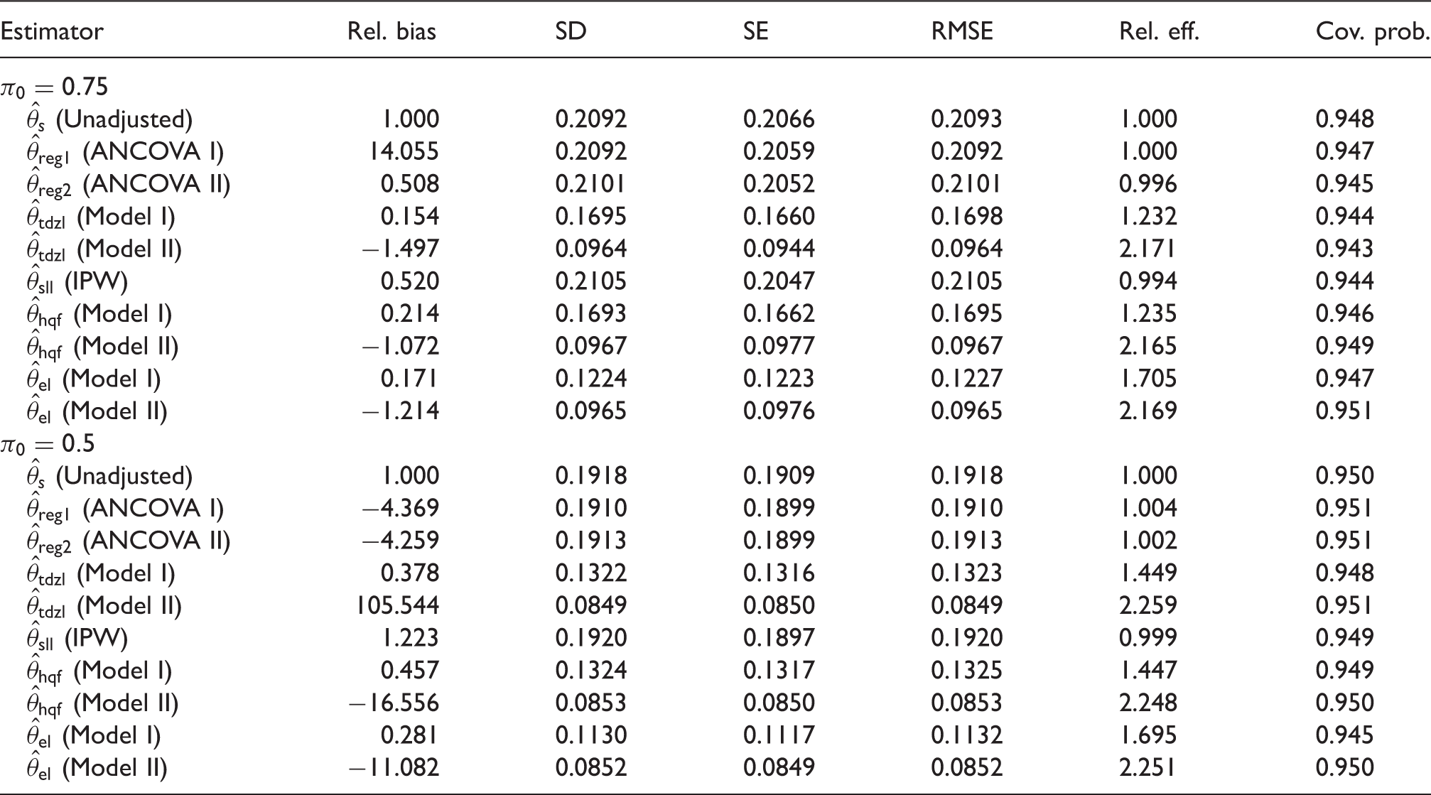
Table 3 reports the simulation results for $(n, π_{0}) = (400, 0.75)$ and $(n, π_{0}) = (400, 0.5)$ , while Table 4 reports the simulation results for $(n, π_{0}) = (800, 0.75)$ and $(n, π_{0}) = (800, 0.5)$ . For each data set, θ and SDs are estimated using the methods described in Section 2 and Table 1. In each case, the simulation replication is 5000. The results in Tables 3 and 4 can be summarized as follows:

The bias of the unadjusted estimator ${\hat{θ}}_{s}$ is identical to 0.0029 for $(n, π_{0}) = (400, 0.75)$ , –0.0012 for $(n, π_{0}) = (400, 0.5)$ , 0.0016 for $(n, π_{0}) = (800, 0.75)$ , and 0.0017 for $(n, π_{0}) = (800, 0.5)$ . The biases of all estimators are negligible, and all the SEs work well. Overall, biases are smaller and SEs estimate SDs better for n = 800 than for n = 400.

As expected, the semiparametric estimators ${\hat{θ}}_{tdzl}, {\hat{θ}}_{hqf}$ , and ${\hat{θ}}_{el}$ perform very similarly and significantly better than other competitors in terms of RMSE under model II, i.e. when the treatment-specific working regression models $m_{1} (X, β_{(1)})$ and $m_{0} (X, β_{(0)})$ are correctly specified. We also observe that these semiparametric estimators have smaller RMSEs under model II for $π_{0} = 0.5$ than for $π_{0} = 0.75$ .

Under model I, i.e. when $m_{1} (X, β_{(1)})$ and $m_{0} (X, β_{(0)})$ are misspecified, the proposed estimator ${\hat{θ}}_{el}$ outperforms the estimators ${\hat{θ}}_{tdzl}$ and ${\hat{θ}}_{hqf}$ in terms of RMSE. By examining the Monte Carlo relative efficiencies, we observe that ${\hat{θ}}_{el}$ has appreciably smaller RMSEs than those of ${\hat{θ}}_{tdzl}$ and ${\hat{θ}}_{hqf}$ under model I. Indeed, ${\hat{θ}}_{el}$ has at least 25% reduction in their RMSEs for $π_{0} = 0.75$ and at least 14% reduction in their RMSEs for $π_{0} = 0.5$ , as compared to ${\hat{θ}}_{tdzl}$ and ${\hat{θ}}_{hqf}$ .

Under model I, the proposed estimator ${\hat{θ}}_{el}$ has considerably smaller RMSEs than those of the other estimators ${\hat{θ}}_{s}$ , ${\hat{θ}}_{reg 1}, {\hat{θ}}_{reg 2}$ , and ${\hat{θ}}_{sll}$ .

The Wald confidence intervals obtained by all the methods attain their coverage probabilities close to the nominal confidence level 0.95. When the sample size is increased from 400 to 800, there is a reduction in coverage error for most confidence intervals.

The performance of the proposed empirical likelihood estimator ${\hat{θ}}_{el}$ is comparable or better than those of the existing estimators when the treatment-specific working regression models are correctly specified and are better than those of the existing estimators when the treatment-specific working regression models are misspecified. In the later case, ${\hat{θ}}_{el}$ has a noticeable reduction in their RMSEs as compared to other estimators.

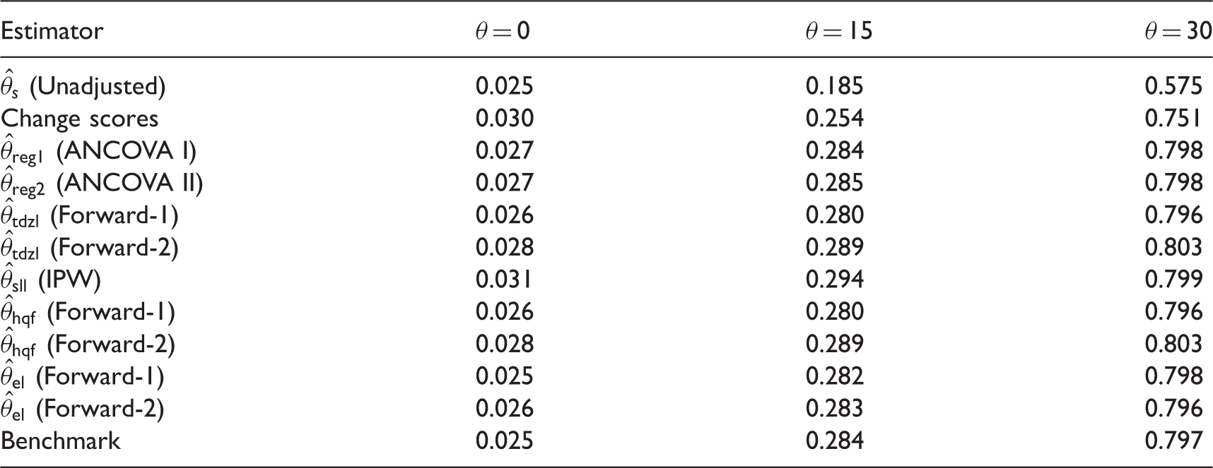
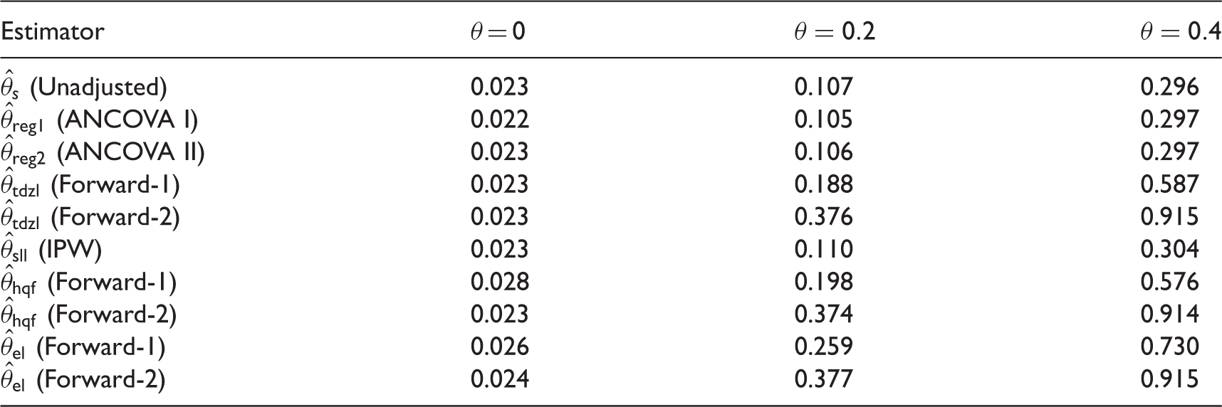
Finally, we investigate the powers of the Wald test statistics produced by all the methods via simulation by testing the null hypothesis

H_{0} : θ = 0

versus the one-sided alternative hypothesis

H_{1} : θ > 0

at significance level 0.025. To this end, we modify the intercept term in the true covariate–outcome relationships by treatment status or

E (Y | D = k, X)

for k = 0, 1, so that the true average treatment effect is identical to

θ = 0, 15, 30

in the first simulation study and

θ = 0, 0.2, 0.4

in the second simulation study. For both scenarios with

(n, π_{0}) = (400, 0.5)

, the achieved significance level and power of each Wald test statistic are calculated as the proportions of rejecting

H_{0} : θ = 0

in favor of

H_{1} : θ > 0

based on 5000 Monte Carlo data sets. The simulation results are summarized in Table 5 for the first simulation study and in Table 6 for the second simulation study. It is seen that the achieved significance levels of all test statistics are quite close to the corresponding nominal significance levels with the exception of the IPW test statistic

{\hat{θ}}_{sll}

, which is notably larger in Table 5 at 0.031, and that the powers of all test statistics are getting larger as θ moves away from 0. For the first simulation study, the powers of

{\hat{θ}}_{reg 1}, {\hat{θ}}_{reg 2}, {\hat{θ}}_{sll}

{\hat{θ}}_{tdzl}, {\hat{θ}}_{hqf}

, and

{\hat{θ}}_{el}

are quite comparable and appreciably larger than the powers of the unadjusted test statistic

{\hat{θ}}_{s}

and the “change scores” test statistic, whereas for the second simulation study, the powers of

{\hat{θ}}_{tdzl}, {\hat{θ}}_{hqf}

, and

{\hat{θ}}_{el}

are notably larger than the powers of

{\hat{θ}}_{s}, {\hat{θ}}_{reg 1}, {\hat{θ}}_{reg 2}, {\hat{θ}}_{sll}

, and the “change scores” test statistic. Our simulation results also reveal that for the second simulation study, the powers of the proposed test statistic

{\hat{θ}}_{el}

are comparable to or higher than those of

{\hat{θ}}_{tdzl}

and

{\hat{θ}}_{hqf}

when the treatment-specific working regression models are correctly specified and are significantly higher than those of

{\hat{θ}}_{tdzl}

and

{\hat{θ}}_{hqf}

when the treatment-specific working regression models are misspecified. In summary, our simulation study indicates that in terms of power performances, the proposed empirical likelihood-based Wald test statistic

{\hat{θ}}_{el}

is comparable to or better than the existing test statistics when the working covariate–outcome relationships by treatment status are correctly specified and are superior to

{\hat{θ}}_{tdzl}

and

{\hat{θ}}_{hqf}

when the working covariate–outcome relationships by treatment status are misspecified.

Table 3.

Relative bias, SD, SE, RMSE, relative efficiency, and coverage probability based on 5000 simulations with sample size $n = 400,$ $Y | X_{1}, X_{2}, D = 1 \sim N (2 + 0.1 X_{1} + 0.2 X_{2} - X_{1}^{2} + X_{2}^{2} + 2 X_{1} X_{2}, 1)$ , $Y | X_{1}, X_{2}, D = 0 \sim N (1 + 0.1 X_{1} + 0.1 X_{2} - 1.2 X_{1}^{2} + X_{2}^{2} + X_{1} X_{2}, 1)$ , and $X_{1}, X_{2} \sim N (0, 1)$ . The incorrect working model I and correct working model II are used.

Estimator	Rel. bias	SD	SE	RMSE	Rel. eff.	Cov. prob.
$π_{0} = 0.75$
${\hat{θ}}_{s}$ (Unadjusted)	1.000	0.2941	0.2916	0.2941	1.000	0.946
${\hat{θ}}_{reg 1}$ (ANCOVA I)	−3.956	0.2939	0.2904	0.2939	1.001	0.945
${\hat{θ}}_{reg 2}$ (ANCOVA II)	0.483	0.2962	0.2886	0.2963	0.993	0.943
${\hat{θ}}_{tdzl}$ (Model I)	0.132	0.2424	0.2343	0.2434	1.209	0.942
${\hat{θ}}_{tdzl}$ (Model II)	22.775	0.1373	0.1340	0.1373	2.143	0.941
${\hat{θ}}_{sll}$ (IPW)	0.447	0.2972	0.2872	0.2972	0.990	0.940
${\hat{θ}}_{hqf}$ (Model I)	0.239	0.2409	0.2352	0.2412	1.219	0.945
${\hat{θ}}_{hqf}$ (Model II)	−2.162	0.1379	0.1433	0.1379	2.133	0.955
${\hat{θ}}_{el}$ (Model I)	0.180	0.1792	0.1776	0.1799	1.635	0.947
${\hat{θ}}_{el}$ (Model II)	−10.853	0.1375	0.1432	0.1375	2.139	0.954
$π_{0} = 0.5$
${\hat{θ}}_{s}$ (Unadjusted)	−1.000	0.2725	0.2698	0.2725	1.000	0.950
${\hat{θ}}_{reg 1}$ (ANCOVA I)	−0.264	0.2716	0.2678	0.2716	1.003	0.948
${\hat{θ}}_{reg 2}$ (ANCOVA II)	−0.268	0.2727	0.2678	0.2727	0.999	0.948
${\hat{θ}}_{tdzl}$ (Model I)	0.197	0.1896	0.1864	0.1897	1.437	0.946
${\hat{θ}}_{tdzl}$ (Model II)	−19.953	0.1206	0.1207	0.1206	2.260	0.946
${\hat{θ}}_{sll}$ (IPW)	−1.190	0.2743	0.2672	0.2743	0.993	0.945
${\hat{θ}}_{hqf}$ (Model I)	0.342	0.1900	0.1866	0.1900	1.434	0.947
${\hat{θ}}_{hqf}$ (Model II)	−2.494	0.1215	0.1208	0.1215	2.242	0.944
${\hat{θ}}_{el}$ (Model I)	0.152	0.1627	0.1587	0.1629	1.672	0.943
${\hat{θ}}_{el}$ (Model II)	−1.696	0.1211	0.1204	0.1211	2.250	0.944

ANCOVA: analysis of covariance; IPW: inverse probability weighting; RMSE: root mean square error; SD: standard deviation; SE: standard error.

Table 4.

Relative bias, SD, SE, RMSE, relative efficiency, and coverage probability based on 5000 simulations with sample size $n = 800,$ $Y | X_{1}, X_{2}, D = 1 \sim N (2 + 0.1 X_{1} + 0.2 X_{2} - X_{1}^{2} + X_{2}^{2} + 2 X_{1} X_{2}, 1)$ , $Y | X_{1}, X_{2}, D = 0 \sim N (1 + 0.1 X_{1} + 0.1 X_{2} - 1.2 X_{1}^{2} + X_{2}^{2} + X_{1} X_{2}, 1)$ , and $X_{1}, X_{2} \sim N (0, 1)$ . The incorrect working model I and correct working model II are used.

Estimator	Rel. bias	SD	SE	RMSE	Rel. eff.	Cov. prob.
$π_{0} = 0.75$
${\hat{θ}}_{s}$ (Unadjusted)	1.000	0.2092	0.2066	0.2093	1.000	0.948
${\hat{θ}}_{reg 1}$ (ANCOVA I)	14.055	0.2092	0.2059	0.2092	1.000	0.947
${\hat{θ}}_{reg 2}$ (ANCOVA II)	0.508	0.2101	0.2052	0.2101	0.996	0.945
${\hat{θ}}_{tdzl}$ (Model I)	0.154	0.1695	0.1660	0.1698	1.232	0.944
${\hat{θ}}_{tdzl}$ (Model II)	−1.497	0.0964	0.0944	0.0964	2.171	0.943
${\hat{θ}}_{sll}$ (IPW)	0.520	0.2105	0.2047	0.2105	0.994	0.944
${\hat{θ}}_{hqf}$ (Model I)	0.214	0.1693	0.1662	0.1695	1.235	0.946
${\hat{θ}}_{hqf}$ (Model II)	−1.072	0.0967	0.0977	0.0967	2.165	0.949
${\hat{θ}}_{el}$ (Model I)	0.171	0.1224	0.1223	0.1227	1.705	0.947
${\hat{θ}}_{el}$ (Model II)	−1.214	0.0965	0.0976	0.0965	2.169	0.951
$π_{0} = 0.5$
${\hat{θ}}_{s}$ (Unadjusted)	1.000	0.1918	0.1909	0.1918	1.000	0.950
${\hat{θ}}_{reg 1}$ (ANCOVA I)	−4.369	0.1910	0.1899	0.1910	1.004	0.951
${\hat{θ}}_{reg 2}$ (ANCOVA II)	−4.259	0.1913	0.1899	0.1913	1.002	0.951
${\hat{θ}}_{tdzl}$ (Model I)	0.378	0.1322	0.1316	0.1323	1.449	0.948
${\hat{θ}}_{tdzl}$ (Model II)	105.544	0.0849	0.0850	0.0849	2.259	0.951
${\hat{θ}}_{sll}$ (IPW)	1.223	0.1920	0.1897	0.1920	0.999	0.949
${\hat{θ}}_{hqf}$ (Model I)	0.457	0.1324	0.1317	0.1325	1.447	0.949
${\hat{θ}}_{hqf}$ (Model II)	−16.556	0.0853	0.0850	0.0853	2.248	0.950
${\hat{θ}}_{el}$ (Model I)	0.281	0.1130	0.1117	0.1132	1.695	0.945
${\hat{θ}}_{el}$ (Model II)	−11.082	0.0852	0.0849	0.0852	2.251	0.950

ANCOVA: analysis of covariance; IPW: inverse probability weighting; RMSE: root mean square error; SD: standard deviation; SE: standard error.

Table 5.

Achieved significance levels and powers of testing the null hypothesis $H_{0} : θ = 0$ versus the alternative hypothesis $H_{0} : θ > 0$ at the level of significance level 0.025 based on 5000 simulations with $(n, π_{0}) = (400, 0.5)$ using the ACTG 175 data.

Estimator	θ = 0	θ = 15	θ = 30
${\hat{θ}}_{s}$ (Unadjusted)	0.025	0.185	0.575
Change scores	0.030	0.254	0.751
${\hat{θ}}_{reg 1}$ (ANCOVA I)	0.027	0.284	0.798
${\hat{θ}}_{reg 2}$ (ANCOVA II)	0.027	0.285	0.798
${\hat{θ}}_{tdzl}$ (Forward-1)	0.026	0.280	0.796
${\hat{θ}}_{tdzl}$ (Forward-2)	0.028	0.289	0.803
${\hat{θ}}_{sll}$ (IPW)	0.031	0.294	0.799
${\hat{θ}}_{hqf}$ (Forward-1)	0.026	0.280	0.796
${\hat{θ}}_{hqf}$ (Forward-2)	0.028	0.289	0.803
${\hat{θ}}_{el}$ (Forward-1)	0.025	0.282	0.798
${\hat{θ}}_{el}$ (Forward-2)	0.026	0.283	0.796
Benchmark	0.025	0.284	0.797

ACTG 175: ACTG Protocol 175; ANCOVA: analysis of covariance; IPW: inverse probability weighting.

Table 6.

Estimator	θ = 0	$θ = 0.2$	$θ = 0.4$
${\hat{θ}}_{s}$ (Unadjusted)	0.023	0.107	0.296
${\hat{θ}}_{reg 1}$ (ANCOVA I)	0.022	0.105	0.297
${\hat{θ}}_{reg 2}$ (ANCOVA II)	0.023	0.106	0.297
${\hat{θ}}_{tdzl}$ (Forward-1)	0.023	0.188	0.587
${\hat{θ}}_{tdzl}$ (Forward-2)	0.023	0.376	0.915
${\hat{θ}}_{sll}$ (IPW)	0.023	0.110	0.304
${\hat{θ}}_{hqf}$ (Forward-1)	0.028	0.198	0.576
${\hat{θ}}_{hqf}$ (Forward-2)	0.023	0.374	0.914
${\hat{θ}}_{el}$ (Forward-1)	0.026	0.259	0.730
${\hat{θ}}_{el}$ (Forward-2)	0.024	0.377	0.915

ANCOVA: analysis of covariance; IPW: inverse probability weighting.

7 Concluding remarks

In this paper, we have proposed an empirical likelihood estimator of the average treatment effect based on two unbiased estimating functions that separate adjustment for covariate effects from estimation of the average treatment effect. The proposed semiparametric procedure can be viewed as another effort at covariate adjustment with the aim of making objective inference in randomized clinical trials. The proposed estimator is at least as efficient as the unadjusted estimator (difference in treatment-specific sample means) and the adjusted estimators of Tsiatis et al.¹ and Huang et al.²² for any given treatment-specific working regression models, and is as efficient as the adjusted estimators of Tsiatis et al.¹ and Huang et al.²² when both treatment-specific working regression models coincide with the true treatment-specific covariate–outcome relationships. We have also made efficiency and power comparisons of the proposed estimator with other existing estimators. The simulation results indicate that the proposed empirical likelihood estimator has competitive finite sample properties in terms of bias, RMSE, and power. The proposed semiparametric approach is illustrated using an analysis of the data from the ACTG 175.

Missing outcomes frequently occur in health science studies. It is of interest to adapt the proposed empirical likelihood method to handle outcome missing at random in randomized clinical trials in addition to covariate adjustment. This is an avenue for further exploration.

Supplemental Material

Supplemental material for Empirical likelihood inference in randomized clinical trials

Supplemental Material for Empirical likelihood inference in randomized clinical trials by Biao Zhang in Statistical Methods in Medical Research

Footnotes

Acknowledgements

I am grateful to the editor and two reviewers for a number of helpful comments and suggestions that have improved my original submission.

Declaration of conflicting interests

The author(s) declared no potential conflicts of interest with respect to the research, authorship, and/or publication of this article.

Funding

The author(s) received no financial support for the research, authorship, and/or publication of this article.

Supplemental material

Supplemental material is available for this article online.

References

Tsiatis

Davidian

Zhang

et al.

Covariate adjustment for two-sample treatment comparisons in randomized clinical trials: a principled yet flexible approach. Stat Med 2008; 27: 4658–4677.

Senn

. Covariate imbalance and random allocation in clinical trials. Stat Med 1989; 8: 467–475.

Koch

Tangen

Jung

et al.

Issues for covariance analysis of dichotomous and ordered categorical data from randomized clinical trials and non-parametric strategies for addressing them. Stat Med 1998; 17: 1863–1892.

Lesaffre

Bogaerts

et al.

On the variability of covariance adjustment: experience with Koch’s method for evaluating the absolute difference in proportions in randomized clinical trials. Control Clin Trials 2002; 23: 127–142.

Lesaffre

Senn

. A note on non-parametric ANCOVA for covariate adjustment in randomized clinical trials. Stat Med 2003; 22: 3583–3596.

Altman

Adjustment for covariate imbalance. In: Armitage

Colton

(eds). Encyclopedia of biostatistics, 2nd ed. Chichester: Wiley, 2005, pp. 1273–1278.

Fleiss

. The design and analysis of clinical experiments, New York: Wiley, 1986.

Leon

Tsiatis

Davidian

. Semiparametric estimation of treatment effect in a pretest-posttest study. Biometrics 2003; 15: 1046–1055.

Davidian

Tsiatis

Leon

. Semiparametric estimation of treatment effect in a pretest-posttest study with missing data (with discussion). Stat Sci 2005; 20: 261–301.

10.

Assmann

Pocock

Enos

et al.

Subgroup analysis and other (mis)uses of baseline data in clinical trials. Lancet 2000; 355: 1064–1069.

11.

Raab

Day

Sales

. How to select covariates to include in the analysis of a clinical trial. Control Clin Trials 2000; 21: 330–342.

12.

Senn

. Consensus and controversy in pharmaceutical statistics. Statistician 2000; 49: 135–176.

13.

Pocock

Assmann

Enos

et al.

Subgroup analysis, covariate adjustment and baseline comparisons in clinical trial reporting: current practice and problems. Stat Med 2002; 21: 2917–2930.

14.

Shen

. Inverse probability weighting for covariate adjustment in randomized studies. Stat Med 2014; 33: 555–568.

15.

Williamson

Forbes

White

. Variance reduction in randomised trials by inverse probability weighting using the propensity score. Stat Med 2014; 33: 721–737.

16.

Horvitz

Thompson

. A generalization of sampling without replacement from a finite universe. J Am Statist Assoc 1952; 47: 663–685.

17.

Owen

. Empirical likelihood ratio confidence intervals for a single functional. Biometrika 1988; 75: 237–249.

18.

Owen

. Empirical likelihood confidence regions. Ann Statist 1990; 18: 90–120.

19.

Qin

Lawless

. Empirical likelihood and general estimating equations. Ann Statist 1994; 22: 300–325.

20.

Hall

La Scala

. Methodology and algorithms of empirical likelihood. Int Stat Rev 1990; 58: 109–127.

21.

Owen

. Empirical likelihood, New York: Chapman & Hall/CRC, 2001.

22.

Huang

Qin

Follmann

. Empirical likelihood-based estimation of the treatment effect in a pretest-posttest study. J Am Stat Assoc 2008; 103: 1270–1280.

23.

Hammer

Katzenstein

Hughes

et al.

A trial comparing nucleoside monotherapy with combination therapy in HIV-infected adults with CD4 cell counts from 200 to 500 per cubic millimeter. N Engl J Med 1996; 335: 1081–1090.

24.

Tsiatis

. Semiparametric theory and missing data, New York: Springer, 2006.

Supplementary Material

Please find the following supplemental material available below.

For Open Access articles published under a Creative Commons License, all supplemental material carries the same license as the article it is associated with.

For non-Open Access articles published, all supplemental material carries a non-exclusive license, and permission requests for re-use of supplemental material or any part of supplemental material shall be sent directly to the copyright owner as specified in the copyright notice associated with the article.

0.00 MB

0.06 MB