






Abstract
Joint modelling of longitudinal and time-to-event data is a powerful tool for analysing complex medical data. Joint latent class models (JLCMs), in particular, provide additional prognostic insight by clustering subjects into latent subgroups within a mixture of experts framework. Traditionally, the mixing proportions are modelled using a multinomial logistic regression. Recent work in mixture regression has proposed a neural network alternative, implemented through the neural network expectation–maximization algorithm, which offers greater flexibility by capturing nonlinearities that may be missed by logistic regression. In this article, we extend the JLCM by applying the neural network to the modelling the mixing proportions captured in the class-membership submodel. The model estimated using an expectation–maximization-type algorithm. We call this the neural-network JLCM (NN-JLCM). We formally define the method, evaluate its performance through extensive simulations, and apply it to real data. The results show that NN-JLCM improves predictive accuracy and class separation compared with traditional JLCMs, while maintaining competitiveness in terms of overall model fit. The code for the article is available at https://github.com/tharris0924/nn-jlcm_p1.
Keywords
Introduction
Longitudinal studies are typically interested in collecting multiple kinds of data on subjects, often a repeated measurement response linked to some event-time of interest, as well as covariates collected at baseline. Examples across multiple disciplines include cognitive assessments recorded repeatedly alongside time to dementia onset or death 1 ; recidivism risk scores derived from supervisor evaluations and time until reincarceration 2 ; mortgage default times paired with current unpaid balances 3 ; longitudinal measures of disability and time to tracheostomy or death in amyotrophic lateral sclerosis trials assessing olesoxime efficacy 4 ; and systemic cytokine biomarkers examined in relation to pneumonia progression and risk of severe sepsis or death. 5
Joint modelling of time-to-event and longitudinal data typically follows one of two methodologies: shared random effects models (SREMs)6,7 and joint latent class models (JLCMs).8–10 SREMs assume that the relationship between risk of event failure is linked to one or more longitudinal responses directly. This allows practitioners to observe the implicit association between biomarkers and the risk of event-failure. This kind of model is one of the more popular approaches to joint modelling with much research in joint models over the past two decades being centred around SREMs6,11,12 with more recent extensions largely considering Bayesian approaches.13–15 However, SREMs may be inadequate when the population under study is heterogenous, that is, made up of homogeneous subpopulations that are typically unobserved. In this case, JLCMs provide a suitable modelling framework.16,17
The JLCM assumes that the time-to-event and longitudinal responses are linked by the hidden heterogeneity in the population in the form of latent classes. This approach draws inspiration from mixtures of experts modelling17,18 where we consider the marginal probabilities of latent classes to be functions of observable baseline covariates, which are then linked to sub-models of the event-time and longitudinal response. 4 This approach has received much attention in terms of extensions for the longitudinal and survival submodels,8,16 but very little research has been done for the class-membership model, which is typically assumed to be a multinomial logistic regression. The exception is Zhang and Simonoff, 17 who considered a tree-based class-membership model, whereby the decision tree would split variables based on a hypothesis test of conditional independence.
The logistic regression model, while useful, requires the validation of the linear parametric assumptions. 19 If the relationship between the cluster-membership and the covariates is nonlinear, then the logistic regression cannot adequately capture this relationship. In the mixture modelling literature, there are studies which consider alternate forms of the class-membership model or mixing proportion function. Young and Hunter 20 considered a nonparametric function of predictors for the mixing proportions, showcasing better performance compared to the standard multinomial logistic regression. Huang and Yao 21 also considered a semiparametric extension whereby the mixing proportions were governed by a kernel regression technique with a local likelihood. Xue and Yao 19 proposed an interesting extension by modelling the mixing proportions by way of a neural network combined with maximum likelihood estimation, yielding superior results than either a kernel-based approach or a traditional logistic regression approach. Furthermore, deep learning has also been used in modelling shared parameter joint models with much success in prognostic predictions.22–24
The JLCM framework is currently only available in Proust-Lima et al., 9 whereby the class-membership model used is a multinomial regression model, with no other readily available competitor. 4 The model is estimated using a Marquardt algorithm, a Newton-like algorithm, but the approach suffers from flexibility issues, in that the class-membership model cannot be replaced with an approach that has been shown to yield improved classification and prediction. The work of Zhang and Simonoff 17 is one such approach, where the authors adopted machine learning for JLCMs, which allows practitioners to consider a non-linear and nonparametric approach for the class membership. By using a tree-based approach, this yielded improved predictive capabilities for the survival and longitudinal model called the joint latent class tree (JLCT). This approach is considered a two-stage modelling approach, where the tree is fit using recursive binary splitting using a hypothesis test as the splitting criterion (similar in fashion to survival trees), and the longitudinal and survival models are fitted separately using Newton-Raphson approaches. However, there is no such unified approach that combines machine learning and maximum likelihood in the estimation of JLCMs to take advantage of the benefits of a hybridized approach.
This article proposes a novel approach for estimating the mixing proportions in a JLCM by using a neural network. An expectation–maximization (EM) algorithm 25 is developed to estimate the model parameters. The advantage of the approach allows practitioners to flexibly model nonlinear relationships between class-membership and the covariates, without relying on parametric assumptions of logistic regressions. This is to say that machine-learning adapted approaches within JLCMs can yield superior clustering solutions and prognostic predictions. These advantages are confirmed by our extensive simulation results and application. As a result, better prognostic predictions of survival and longitudinal outcomes are possible using the neural network for the class-membership. This, in turn, leads to more robust clustering solutions in the face of increasingly complex disease modelling.
The rest of the article is organized as follows. Section 2 considers the materials and methods needed for the study by giving a background on joint modelling, JLCM and our proposed method using deep learning. Section 3 details an extensive simulation study where the proposed neural-network JLCM (NN-JLCM) consistently outperforms the traditional JLCM across three simulation studies. Additional tables and simulation results are given in the Supplemental Material. In Section 4, NN-JLCM is compared with JLCM, the JLCT of Zhang and Simonoff, 17 and SREM of Rizopoulos 26 across additional experiments to further assess the finite sample properties of the NN-JLCM method. The first such experiment is where all the simulations are repeated from Section 3, but now an array of models is fitted with varying chosen latent classes. We report on the latent class selection criteria to determine the model’s efficacy at selecting the correct number of latent classes. The second experiment considers fitting the models to a dataset with considerable cluster overlap. The final experiment considers a double-fold evaluation of the assumptions of the NN-JLCM, where in the first instance, we generate from an SREM and fit the NN-JLCM to the data, and in the second instance, we generate from a JLCM and fit the NN-JLCM to the data. This is to evaluate the robustness of the NN-JLCM in the face of model misspecification. Section 5 considers an application of the model to the PAQUID dataset, 27 where the longitudinal measure we consider is the normalized mini-mental state examination (MMSE) and the event-time we consider is dementia. We show that NN-JLCM has superior predictive capabilities for both the longitudinal and survival outcomes, while also yielding better class separation compared to the JLCM, JLCT, and SREM. In Section 6, after discussing the results obtained, we conclude the article and provide direction for future research.
Materials and methods
A brief primer on time-to-event and repeated measurement analysis
Let the random variable




In addition to survival times, there might be other measurements made on the subject over time. Let


Unlike the SREMs, the JLCM does not directly link the time-to-event model and linear mixed-effects model with an association parameter. Instead, the assumption is that the association between the time-to-event and longitudinal processes is captured by the predicted latent classes.9,10 Every latent class has a class-specific repeated measurement trajectory and a class-specific hazard function. The JLCM draws inspiration from finite mixture modelling, specifically, finite mixtures of experts. 18
Fundamentally, it is also assumed that the repeated measurements and the time-to-event are independent conditionally on the latent class. The reasoning for this: it is conjectured that the observed association between the time-to-event and longitudinal data over the entire population is spurious, largely driven by the heterogeneity in levels of the variables between latent classes. 17
Let the

The class-specific linear mixed-effects model is given as follows:

The
The class-specific hazards function is given by the following equation:

Let

The likelihood in equation (8) is maximized using an extended Marquardt algorithm, a Newton-type algorithm with stringent convergence criteria.9,31 In the extended Marquardt algorithm, the parameter vector


Convergence is declared when three conditions are simultaneously satisfied. The first is for parameter stability, the second is for log-likelihood stability, and the last one is a derivative-based criterion for the relative distance to the maximum. The variance-covariance matrix of the estimates, denoted
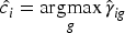
Classification with the model is performed using the posterior conditional probabilities, or responsibilities, which are computed as follows:

Using equation (11), we can determine the model-based clusterings based on the predicted responsibilities, as follows:

Finally, the JLCM assumes that the latent class structure fully captures the dependency between the longitudinal marker(s) and the time-to-event. Several methods can be used to evaluate this assumption, including posterior classification analysis, residual analysis, and a score test.
4
In the score test, the alternative hypothesis

Testing conditional independence reduces to

Here we consider our proposed model. The model parameterizations for the longitudinal and survival submodels remain the same. In this article, we consider a neural network to model the mixing proportions
Neural networks
Neural networks are inspired by the way in which information travels and is stored in the human brain. This is where neurons, the most basic processing unit of the brain, would ‘fire’ by sending electrical impulses along neural pathways to connect to other neurons through synaptic links (or synapses).
There are approximately 90 billion neurons and 100 trillion synapses in the human brain, where each neuron is connected through several thousand synapses. As a neuron receives information from another neuron, it can be induced to fire as well, through signals known as neurotransmitters, which are released at the synapses. Certain synaptic pathways inhibit or exacerbate the neural impulse so that firing an input neuron will reduce the likelihood of the output neuron firing. 33
Mathematical properties of neural networks were first pioneered by McCulloch and Pitts
34
with the first simplistic neural network models such as the perceptron studied in the seminal work of Rosenblatt.
35
Mathematically, the output of the


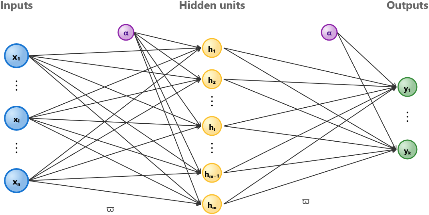
Architecture for a single hidden-layer neural network.
Estimation of the weights and biases is done using a variant of gradient descent and back-propagation, which seeks to minimize the following function:

Backpropagation is an algorithm that computes gradients of the loss function with respect to the network parameters (weights












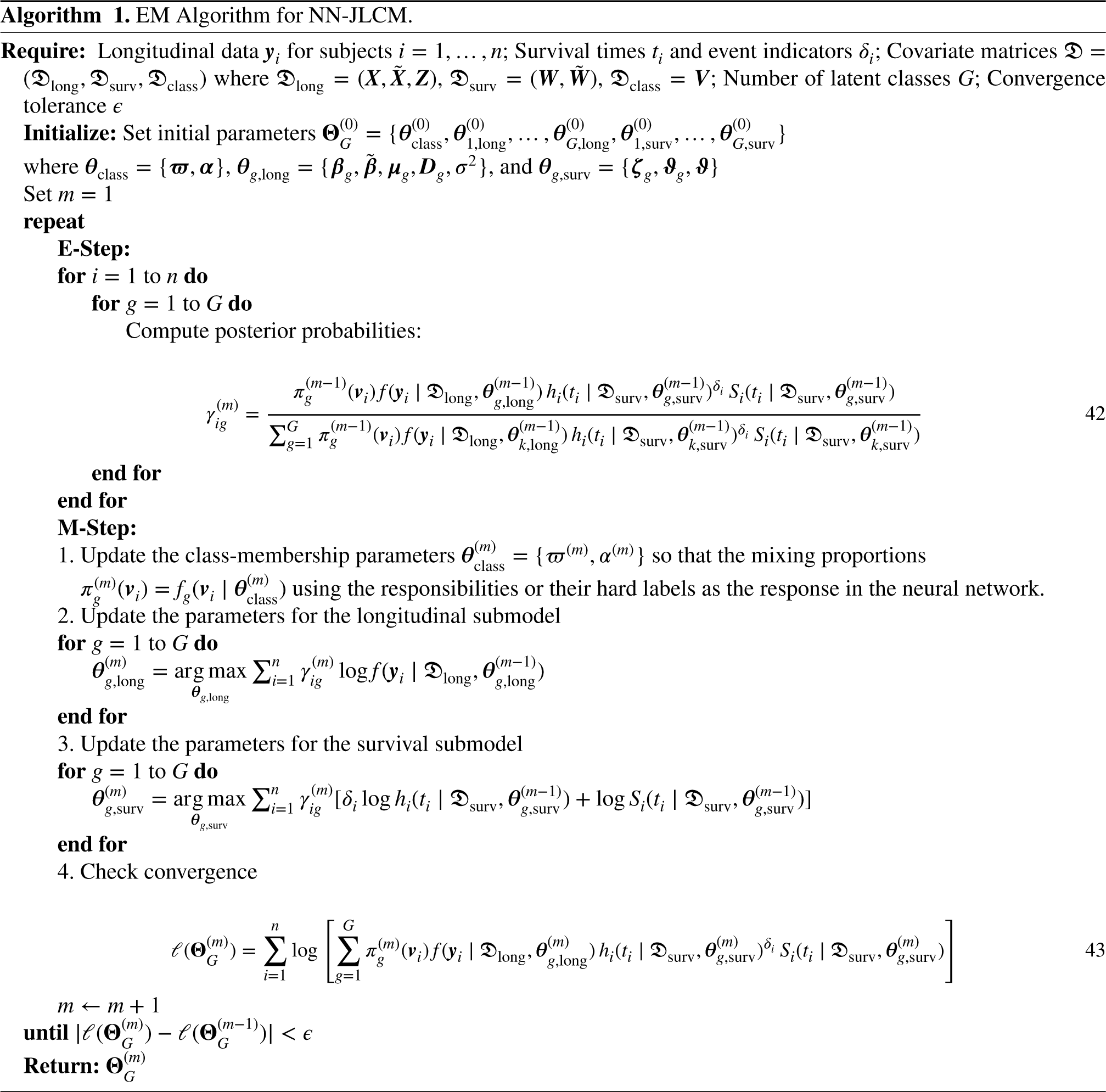
The NN-JLCM is our proposed model, and we use an EM algorithm to estimate the parameters of the model. The structures of the longitudinal submodel in equation (6) and the survival submodel in equation (7) remain the same. We begin by briefly describing the EM algorithm and then giving the complete data log-likelihood, and then proceed to the E-steps and M-steps, respectively.
Brief description of the EM algorithm
The EM algorithm, first introduced by Dempster et al., 25 is a highly versatile iterative algorithm developed to estimate the maximum likelihood in the context of incomplete data problems. This can include both natural incomplete data problems, where we have censoring, for example, or an artificial incomplete data problem, such as the unknown latent class in finite mixture models. The problem is usually solved by introducing the missing data as a latent variable, resulting in complete data. The logic is that the log-likelihood of the complete data is typically easier to maximize, often in a closed form. The algorithm has two steps: the expectation (E-), where we calculate the expected value of the complete data log-likelihood. The second step of the EM algorithm is to maximize (M-) the expected complete-data log-likelihood function obtained in the E-step. The E- and M-steps are repeated until convergence. A very brief description of how it works follows.
Assuming that we have our complete data matrix represented by

We then update the parameters in the M-step by the following equation:

We now define the NNEM algorithm for estimating the NN-JLCM. As equation (8) is the observed log-likelihood of the JLCM, the complete data log-likelihood can be written using the notation established. Let the unobserved indicator
Additionally, let the observed covariates comprising the design matrices for the longitudinal, survival, and class-membership submodels be denoted as
Let


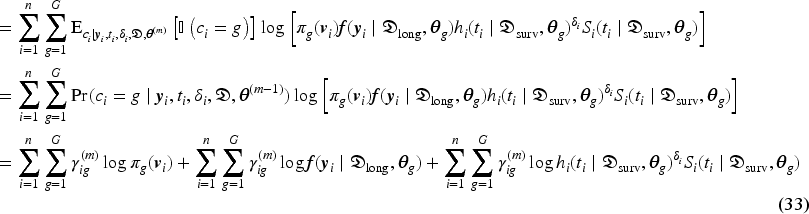
To update the mixing proportions


Let

For the survival submodel, let Neural network joint latent class model (JLCM) framework where the gating network is captured by a neural network as opposed to a multinomial model in the classical JLCM implementation.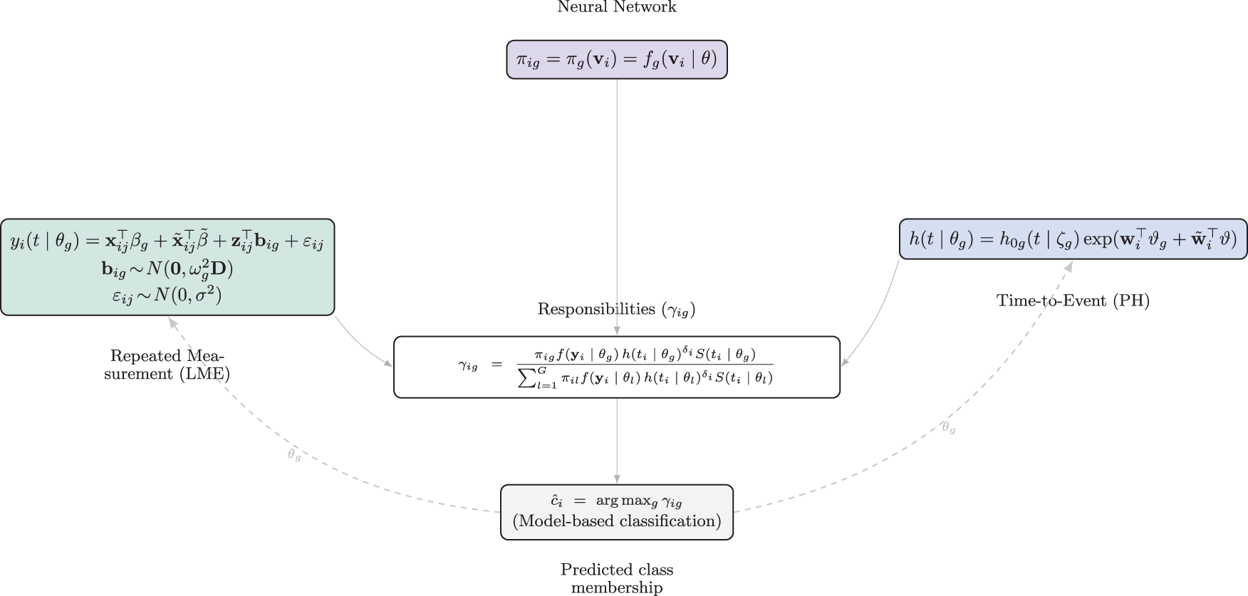


The model parameters at each iteration


When the optimization problem admits a unique solution, convergence to the minimum is guaranteed regardless of the initial parameter values.
The parameters of the neural network model are estimated using gradient descent as explained above.33,40 To summarize the NN-JLCM approach, we give the full algorithm in Algorithm 1 and showcase the intuition of the modelling approach in Figure 2.
We have assumed thus far that the number of latent classes is known, however, in practice, this is often unknown. In the latent class joint modelling literature, like in mixture modelling, there is unfortunately no one criteria for determining the number of classes, but a compromise among several criteria. Indeed, the resulting model with the ‘optimal’ number of classes tends to be the model which does not satisfy only one criteria, but a compromise among information criteria, classification meaningfulness and a valid conditional independence assumption as noted by Kyheng et al. 4 and Proust-Lima et al.9,10 For a model to have a valid conditional independence assumption, the score test of conditional independence should not be significant. 32
The information criteria, that is, the Bayesian information criterion (BIC)
41
and the Akaike information criterion (AIC)
42
are defined, respectively, as follows:


The integrated classification likelihood (ICL) of the model is computed as follows
9
:

Further, we compute a measure of entropy
10
alongside the ICL as another metric of classification ability. The metric is computed as follows:

Finally, the responsibilities are used to evaluate the adequacy of the model through an a posteriori classification table. Each individual is assigned to the class corresponding to the largest responsibilities. For each class
In this section, we demonstrate the performance of the proposed estimation procedure for fitting the proposed NN-JLCM (combination of neural network and EM algorithm) compared to the traditional JLCM (combination of logistic model and Marquardt algorithm) approach. We consider
Mean posterior class-membership probabilities by final class assignment.
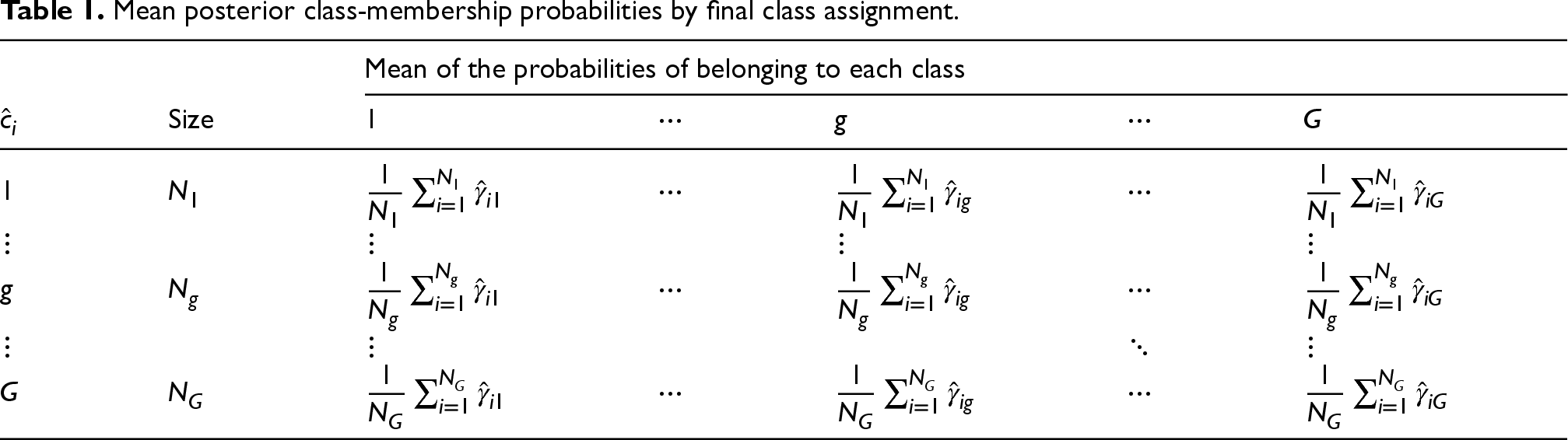
Mean posterior class-membership probabilities by final class assignment.
To assess the finite sample behaviour of the estimates, we compute the absolute bias (AB) and the mean squared error (MSE). The AB of the 

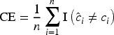
The proposed model’s classification capability is also assessed by computing the classification error (CE) as follows:


For time-to-event predictions, we use the integrated squared error (ISE) to measure the divergence between the true and the predicted survival curves. The ISE for a sample of 
Data-generating process (DGP)
The settings of the first scenario are based on Kyheng et al., 8 where the authors considered a scenario inspired by a real dataset from Stamenic et al., 45 who used a JLCM as a prognostic tool for the prediction of graft failure in patients who are at risk of kidney graft loss. Stamenic et al. 45 considered the serum creatine (SCr) as the longitudinal measurements of interest, and the time-to-event of interest was the onset of de novo donor-specific anti-HLA antibodies. Early prediction of graft failure in kidney transplants is crucial to assess the long-term success of kidney transplants.
We assume that the true survival times 
Varying parameters of the censoring distribution depending on censoring rate.

To simulate the longitudinal profiles of the SCr trajectories, we consider the following class-specific linear mixed-effects model with a random intercept

We can group the fixed effects into vectors 
We assume that the individual number of recordings (
To consider the effect of a mixing proportion which does not conform to assumptions of a monotonic linear function of a logistic regression, we consider the work of Huang and Yao,
21
where the mixing proportions are governed by a sinusoidal function

We have included the table of estimates under light censoring in Table 3 for 1000 simulations. The results for moderate and heavy censoring are included in Supplemental Tables S1 and S2, respectively. The performance for the model estimates of the submodels is similar across both methods, with similar estimate values, biases and MSEs. By increasing the sample size, the MSEs decrease; however, by increasing the censoring rate, the MSEs increase. Additionally, we plot the estimated mixing proportions for the NN-JLCM and JLCMM overlaid on the true mixing proportions in Figure 3.
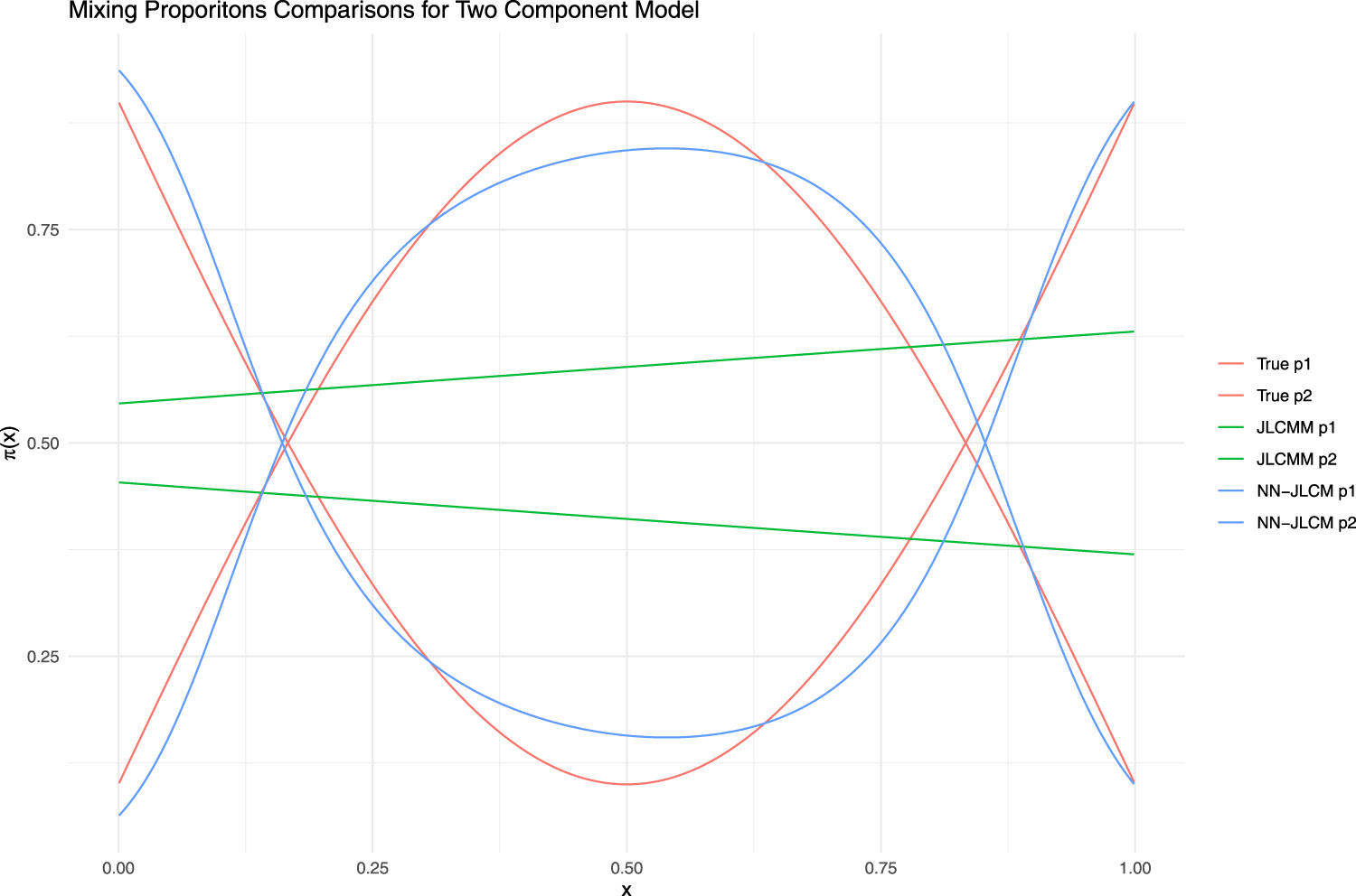
Mixing proportion comparisons for two-component model.
Bias and MSE results for NN-JLCM
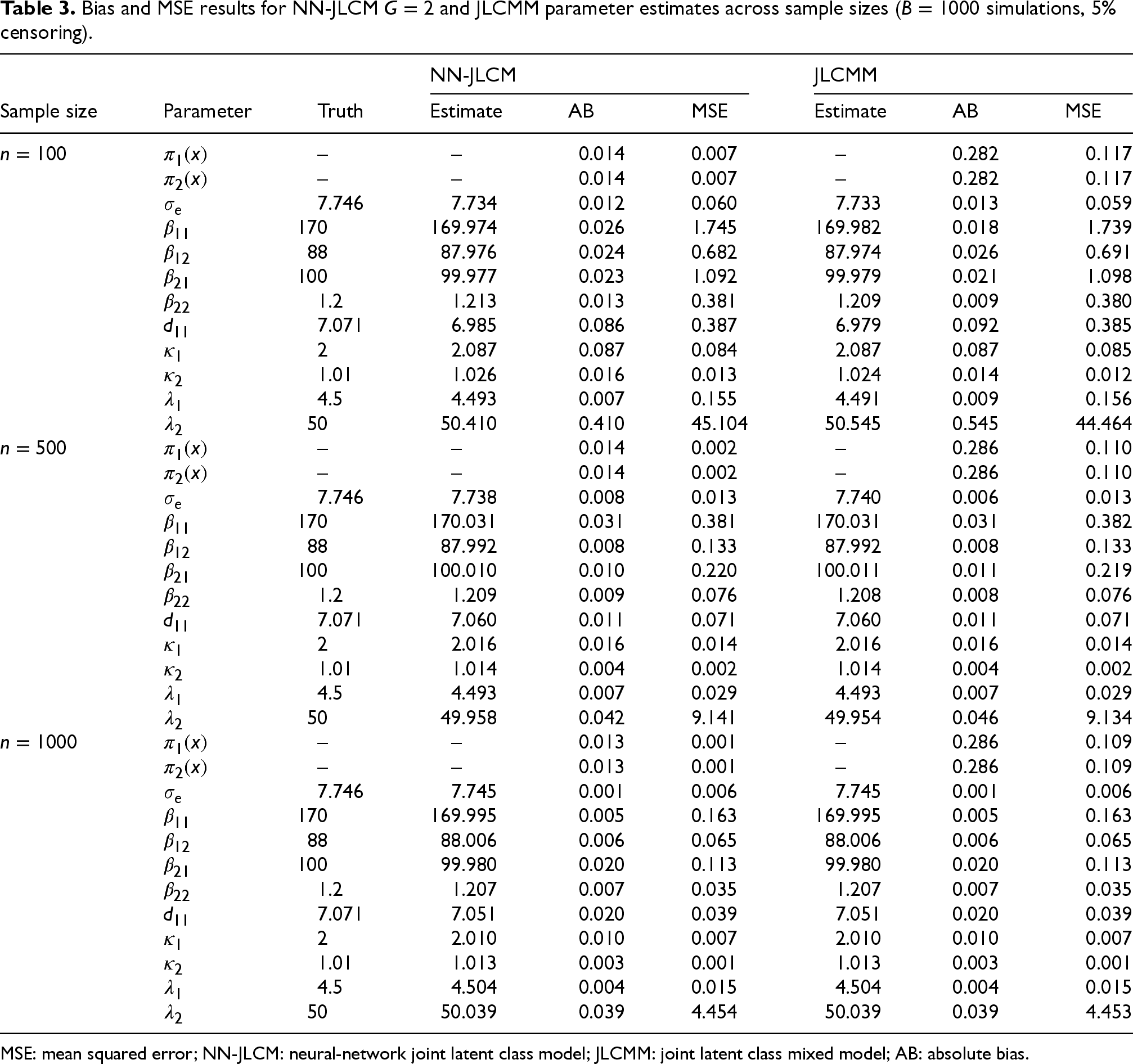
MSE: mean squared error; NN-JLCM: neural-network joint latent class model; JLCMM: joint latent class mixed model; AB: absolute bias.
From Figure 3, we see that the JLCMM approach cannot handle the sinusoidal function as it does not conform to the assumptions of a logistic regression. This leads to biases in the classifications of the model. If the function for the mixing proportions is incorrect, then the posterior classifications naturally suffer. The neural network classification membership function of the NN-JLCM, however, performs quite well and captures the sinusoidal shape of the true function in equation (51), naturally leading to superior classification performance. This is confirmed by the AB and MSE of mixing proportion being much smaller relative to JLCMM across all sample sizes and rates of censoring in Table 3 and Supplemental Tables S1 and S2.
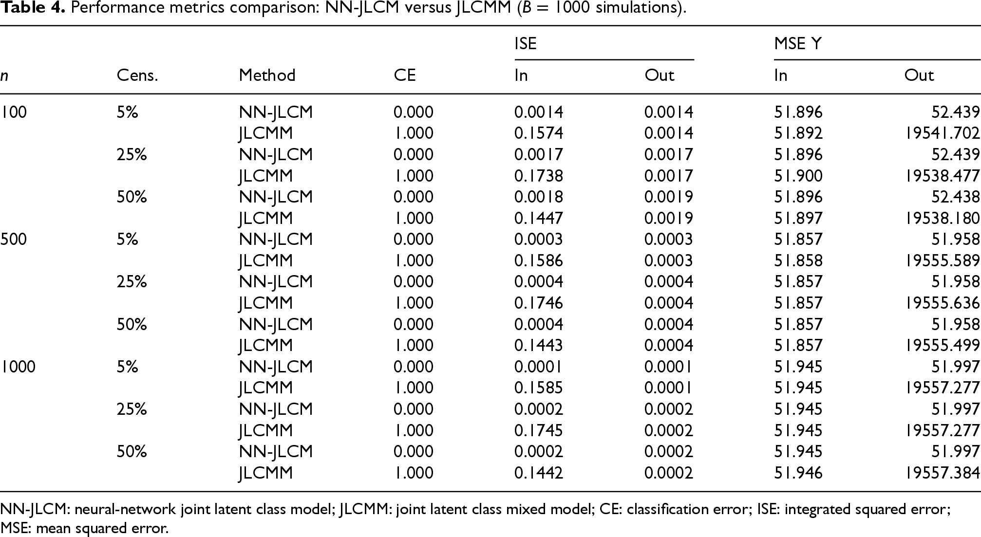
Finally, we computed the average misclassification error and the average prediction errors of the survival curves and longitudinal profiles over all
Performance metrics comparison: NN-JLCM versus JLCMM (
NN-JLCM: neural-network joint latent class model; JLCMM: joint latent class mixed model; CE: classification error; ISE: integrated squared error; MSE: mean squared error.
The ISEs and MSEs are reported for both in-sample and out-of-sample data. The out-sample data had the same rate of censoring and number of subjects as the in-sample data. We can see that the in-sample performance of the JLCMM for ISE is quite poor relative to NN-JLCM across the study. The out-of-sample performance, interestingly, seems to be roughly equivalent between the two methods. The overall performance seems to improve slightly as
For the prediction error, the in-sample performance is roughly equivalent across the methods, whereas the out-of-sample prediction error for JLCMM exhibits serious numerical issues, being more than 100 times greater than NN-JLCM. Increasing the sample size improves the performance slightly for both methods, considering only the in-sample cases. However, the out-of-sample performance actually seems to worsen for JLCMM as we increase the sample size, while the MSE improves for NN-JLCM.
This particular simulation setting showed that the NN-JLCM method is superior to the JLCMM method under varying forms of censoring for the mixing proporitons leading to better predictive and classification performance for NN-JLCM. Next, we will consider the case of three latent classes.
Data-generating process
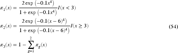
For the second simulation scenario, we consider a three-component model with a more complex mixing proportion taken from Xue and Yao.
19
The mixing proportions are as follows:




Finally, we assume that the survival times are Weibull distributed with scale
Varying parameters of the censoring distribution depending on censoring rate for three-component model.

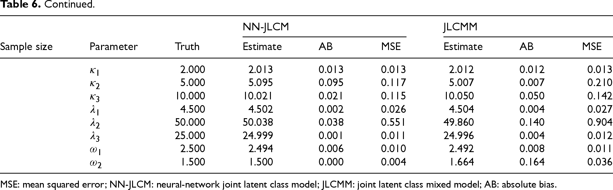
In Table 6, we report the results of our 1000 samples generated using the DGP above under 5% censoring. The results for 25% and 50% censoring are reported in Supplemental Tables S3 and S4, respectively.
Bias and MSE results for NN-JLCM
and JLCMM parameter estimates across sample sizes (
simulations, 5% censoring).
Bias and MSE results for NN-JLCM
MSE: mean squared error; NN-JLCM: neural-network joint latent class model; JLCMM: joint latent class mixed model; AB: absolute bias.
The performance of the estimates of the longitudinal model for NN-JLCM seems to be roughly equivalent to JLCMM, showcasing equivalent MSEs as
In Figure 4, we plotted the fitted mixing proportions
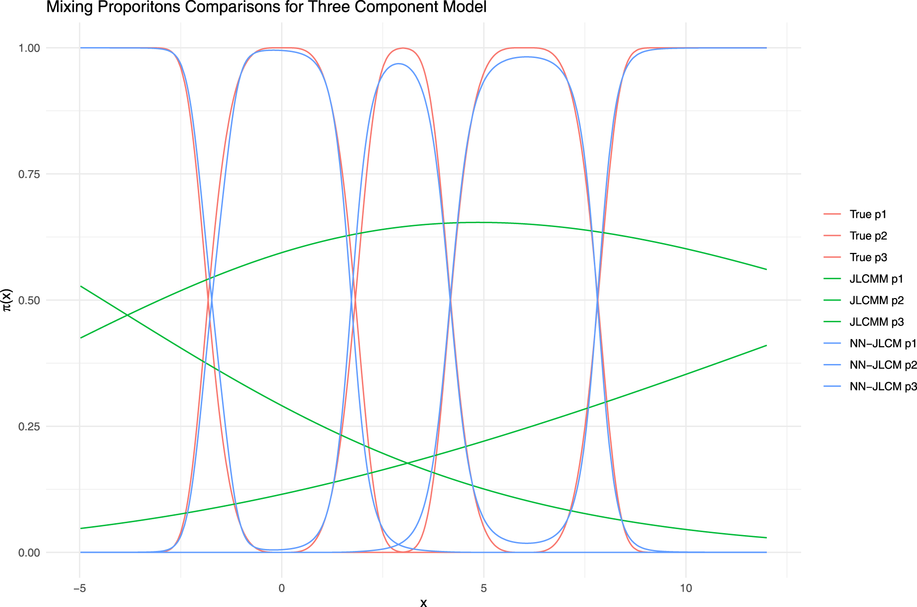
Mixing proportion comparisons.
Finally, in Table 7, we report the prediction errors for the survival curves and longitudinal profiles and the CEs. CEs for JLCMM and NN-JLCM are similar to before, with NN-JLCM greatly outperforming JLCMM. As the level of censoring increases (i.e.
Performance metrics comparison
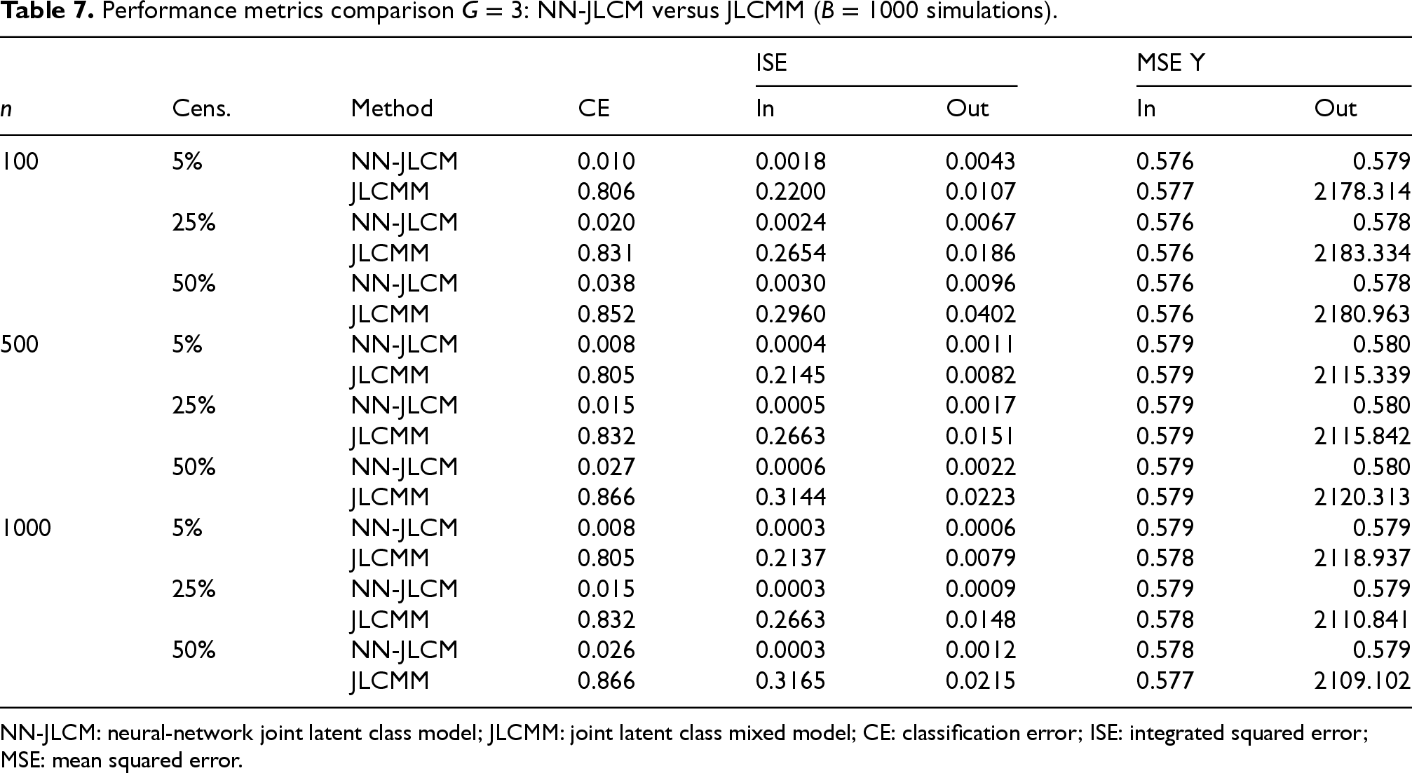
NN-JLCM: neural-network joint latent class model; JLCMM: joint latent class mixed model; CE: classification error; ISE: integrated squared error; MSE: mean squared error.
In this scenario, we see that NN-JLCM once again outperforms JLCMM in predictive accuracy and parameter stability across censoring rates and sample sizes. In the next scenario, we consider a four-component model.
Data-generating process
For the third Scenario, we consider a four-component model with complex mixing proportions extending the framework from Xue and Yao.
19
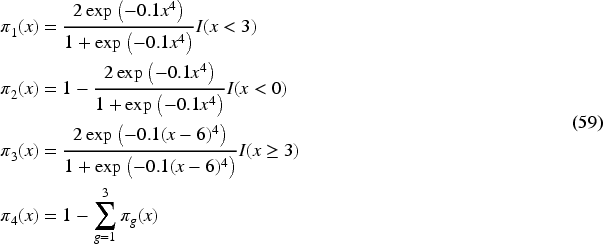
The mixing proportions are as follows:

The true parameters of the survival and longitudinal submodels are inspired by the PAQUID dataset. The PAQUID dataset consists of a random subsample of 500 subjects from the study of a French cohort about dementia and Alzheimer’s incidence rates.
27
The objective here is to jointly model the repeated measurements of scores for the MMSE, which is an assessment of cognitive performance, and the event times for dementia occurrence. We simulate synthetic data for MMSE using the following longitudinal submodel structure:

The true variance parameter is given as 

We assume that the right-censored times
Varying parameters of the censoring distribution depending on censoring rate for four-component model.

Bias and MSE results for NN-JLCM
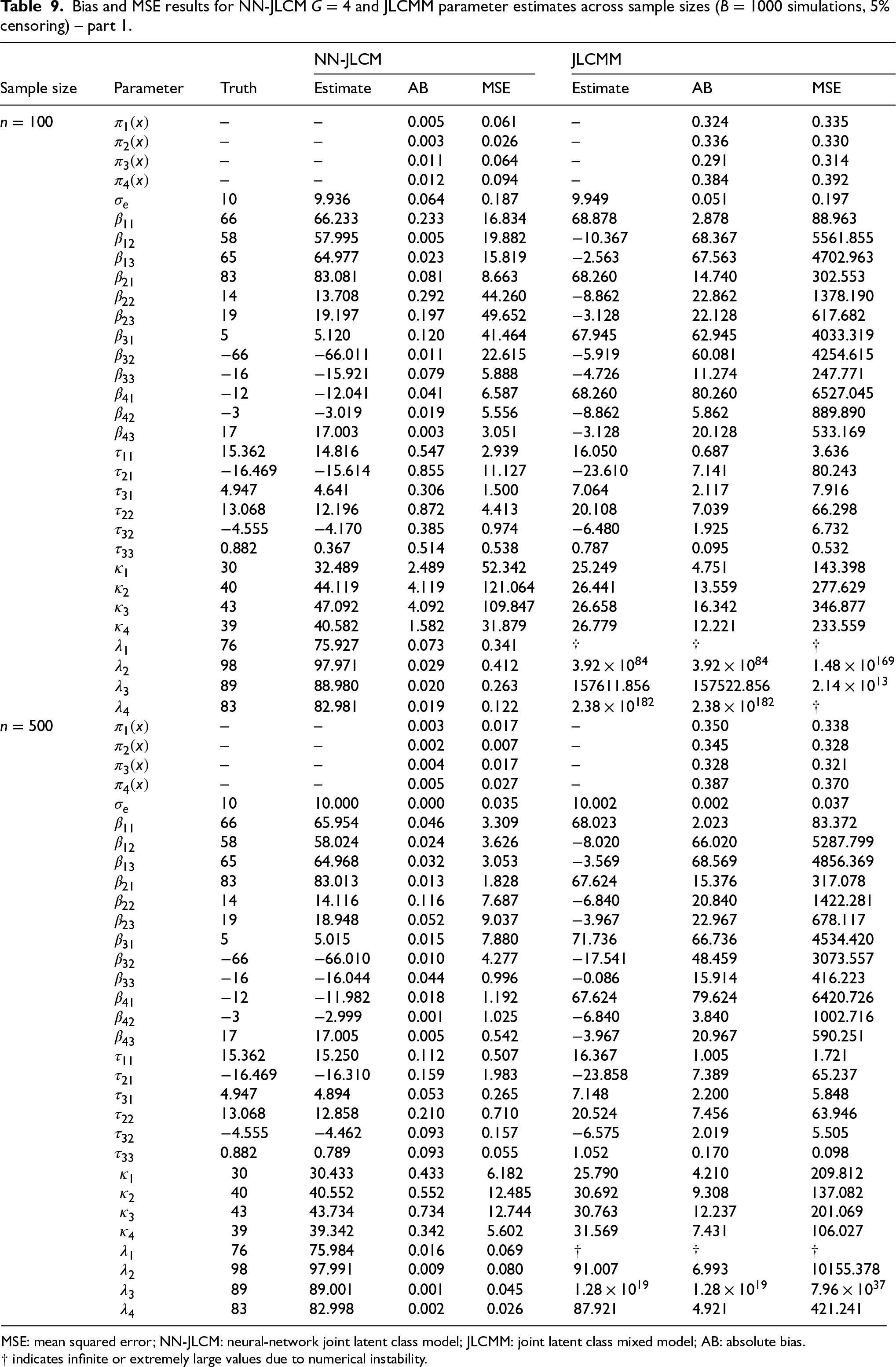
MSE: mean squared error; NN-JLCM: neural-network joint latent class model; JLCMM: joint latent class mixed model; AB: absolute bias.
Bias and MSE results for NN-JLCM
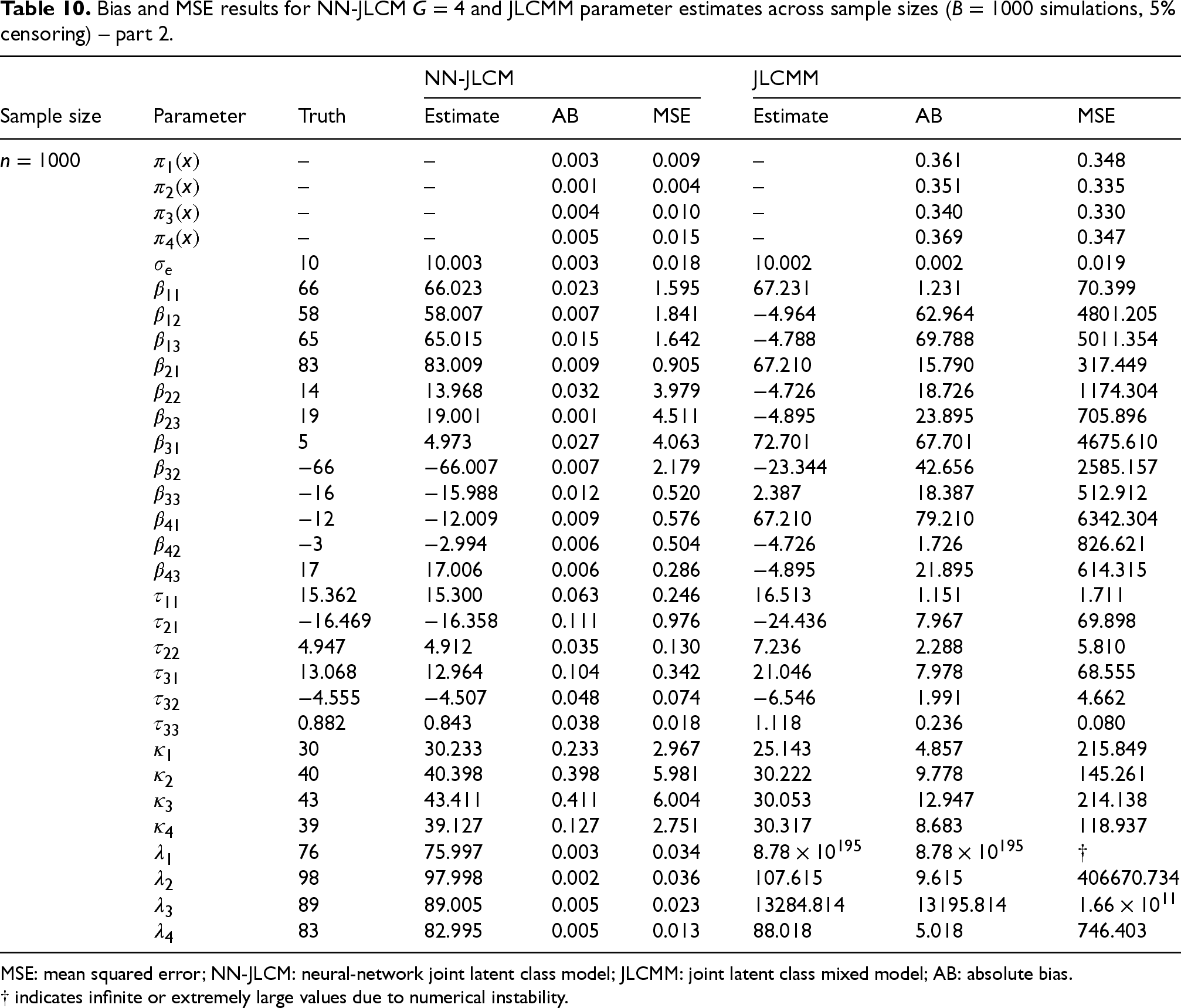
MSE: mean squared error; NN-JLCM: neural-network joint latent class model; JLCMM: joint latent class mixed model; AB: absolute bias.
The results for 5% censoring for
The performance of the estimates of the longitudinal model for NN-JLCM appears to be roughly equivalent to JLCMM, showcasing comparable MSEs as
The survival parameter estimates for JLCMM exhibit severe numerical instability, particularly evident in the extreme values marked with
In contrast, NN-JLCM maintains accurate parameter estimates throughout all sample sizes and censoring rates in this scenario. The MSEs and biases for NN-JLCM show the expected decrease as sample size increases. This stability is particularly noteworthy given the complexity of the four-component model with its highly non-monotonic mixing proportions.
The mixing proportion estimates reveal the core advantage of making use of a neural network-based class-membership model. The NN-JLCM achieves lower bias and MSE values compared to the JLCMM, which barely improves with increased sample size. By looking at Figure 5, this showcases the poor performance of the logistic regression class-membership model of the JLCMM to capture the complex pattern of the true mixing proportions, which propagates through to all other parameter estimates in the JLCMM model.
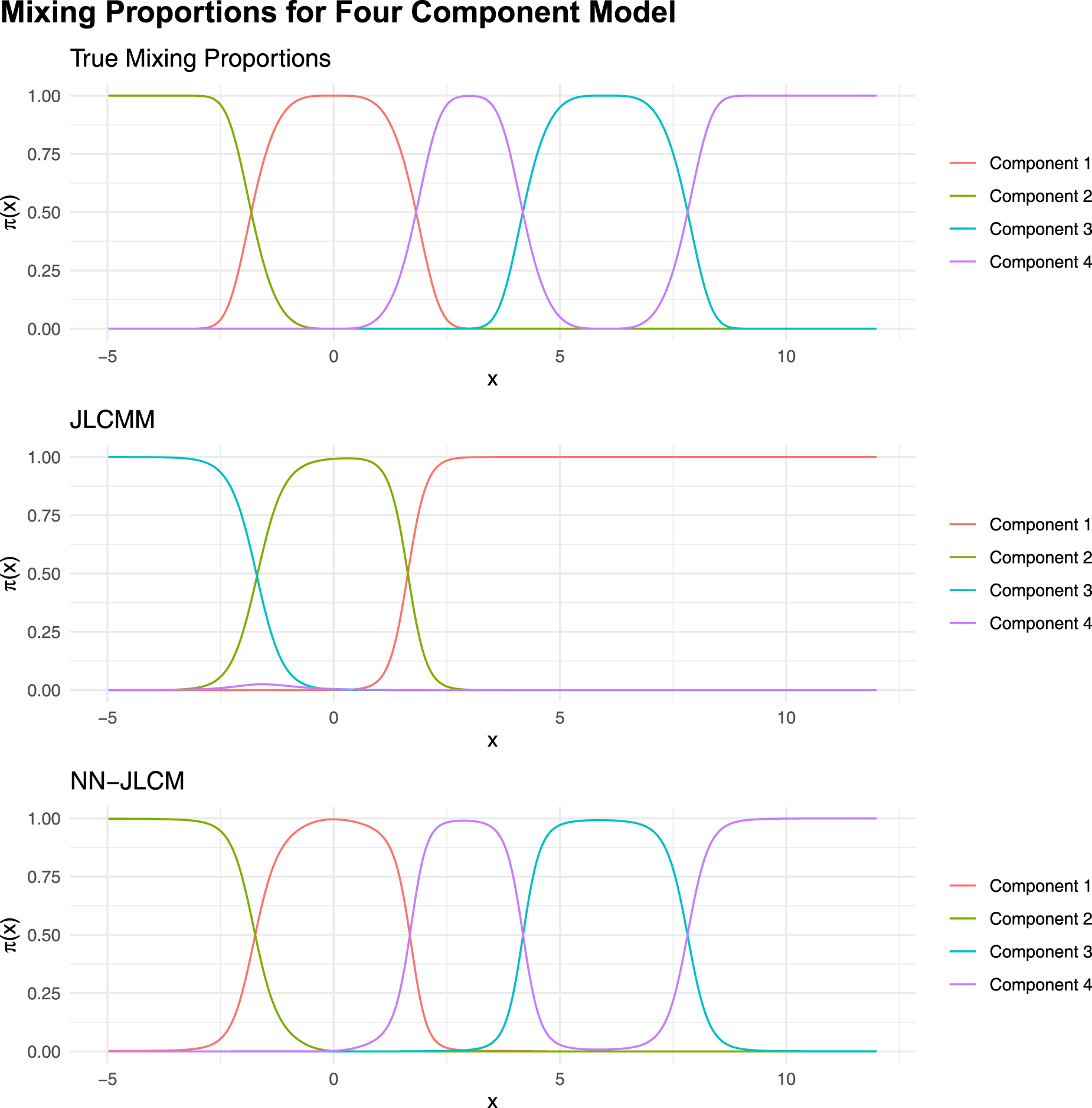
Mixing proportion comparisons for four-component model.
Finally, examining Table 11, the performance metrics demonstrate the practical consequences of these estimation differences. The NN-JLCM achieves near-perfect classification with misclassification errors ranging from 0.005 to 0.017 across all scenarios, while JLCMM exhibits poor classification performance with errors between 0.756 and 0.794. The ISE and MSE metrics follow similar patterns, with NN-JLCM showing superior predictive accuracy for both survival curves and longitudinal trajectories. The out-of-sample prediction errors for JLCMM are large, often exceeding 500 times those of NN-JLCM, indicating potential overfitting and poor generalization capability.
Performance metrics comparison: NN-JLCM versus JLCMM (
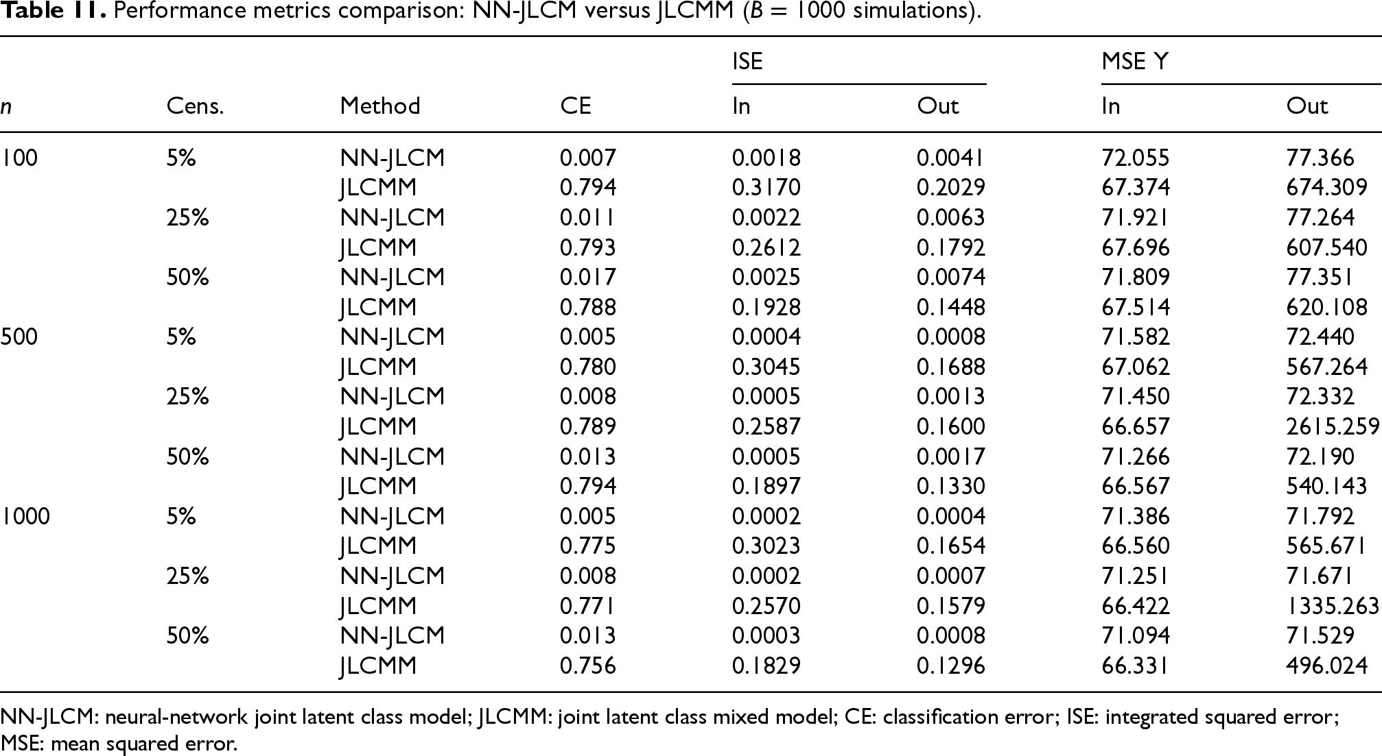
NN-JLCM: neural-network joint latent class model; JLCMM: joint latent class mixed model; CE: classification error; ISE: integrated squared error; MSE: mean squared error.
This four-component scenario represents the most challenging test case, and the results clearly demonstrate that NN-JLCM provides a robust and flexible alternative to traditional JLCMM when the mixing proportions deviate significantly from logistic regression assumptions.
In this section, we conduct a series of simulation experiments to evaluate the performance of the proposed NN-JLCM against the standard JLCM, the SREM implemented in the
Survival and longitudinal submodel predictive assessments
To assess survival curves, we use the integrated Brier score (BS) for censored data. Let 

In addition to the JLCMM and the proposed model, the NN-JLCM, we consider alternate joint modelling techniques for the application. The first among these we consider is the SREM, which is a popular approach for jointly modelling time-to-event processes and longitudinal processes when the direct association between the two is of interest. This is due to the hazard function incorporating an additional term for the mean of the longitudinal profile, allowing us to compute the effect on the risk of event-failure under a marginal increase in the subject-specific mean profile. We use the well-established
Secondly, we consider the JLCT proposed by Zhang and Simonoff. 17 The reason for this is that it is the only other joint latent class modelling approach which considers an embedded machine learning approach for the class-membership submodel. The approach fits a decision tree to the data to find latent class partitions according to the assumption of conditional independence within latent classes. The decision tree recursively does this using a log-likelihood ratio test to verify statistical independence using the extended Cox model which includes the longitudinal measurement of interest within each node. If the parameter on the longitudinal measurement is not significantly different from zero, then it means that there is statistical independence within obtained partition. The goal is to find segments of the data in which the children’s nodes are more homogeneous than their parent nodes to conform to statistical independence within the clusters. Once these partitions are obtained, they are used to fit a separate survival regression model with class-specific parameters and a linear mixed-effects model with class-specific random effects and independent subject-specific random effects. Additionally, JLCT allowed for time-varying latent classifications. The JLCT showcased superior predictive performance and modelling flexibility when compared to SREM and JLCM in a simulation study and an application to PAQUID.17,48 For further information about JLCT, we refer the reader to the work of Zhang and Simonoff17,48 and Fu and Simonoff. 49
Multiple-
simulation
In this simulation, we consider a similar approach to Nguyen and McLachlan
50
of showcasing the efficacy of various metrics in recommending the true number of clusters. We use the true parameters for the three simulation studies discussed in Section 3 to generate data for true
Cluster selection frequency over 1000 simulations.
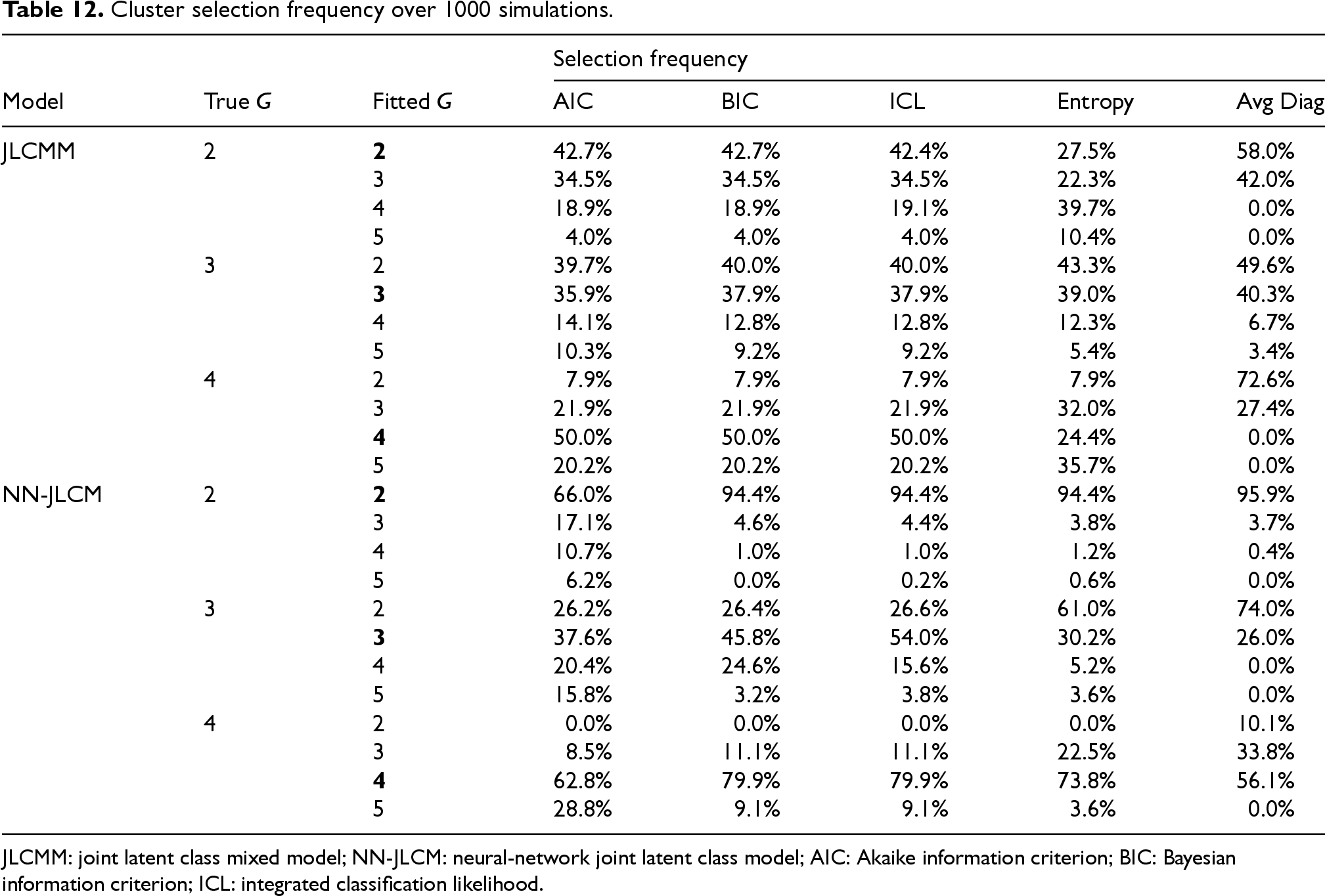
Cluster selection frequency over 1000 simulations.
JLCMM: joint latent class mixed model; NN-JLCM: neural-network joint latent class model; AIC: Akaike information criterion; BIC: Bayesian information criterion; ICL: integrated classification likelihood.
Average simulation metrics by model and true
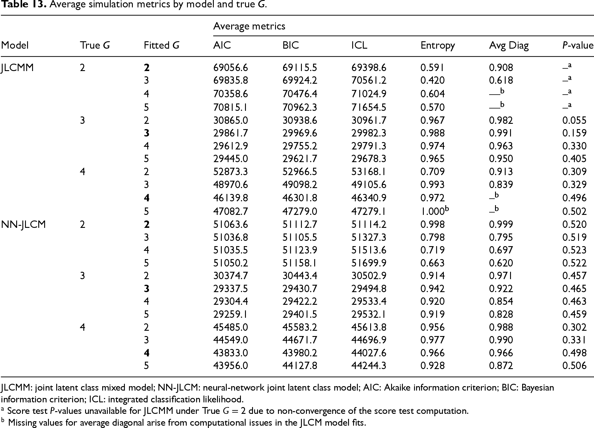
JLCMM: joint latent class mixed model; NN-JLCM: neural-network joint latent class model; AIC: Akaike information criterion; BIC: Bayesian information criterion; ICL: integrated classification likelihood.
The cluster selection frequency table in Table 12 reveals a clear distinction in model selection consistency between JLCMM and NN-JLCM. When the true number of clusters is 2, NN-JLCM demonstrates strong recovery across all information criteria, with BIC, ICL, entropy, and Avg Diag all selecting the correct model over 94% of the time. For JLCMM, AIC, and BIC select the true model less than half the time, and entropy selects
For
For JLCMM with true
The P-values hover around 0.5 for NN-JLCM across most scenarios, regardless of the fitted
Overall, the results suggest that NN-JLCM provides more reliable model selection metrics, particularly in scenarios with well-separated classes, while JLCMM struggles to identify the correct number of clusters due to poor class separation and convergence issues.
To assess the robustness of the NN-JLCM under weak class separation, we consider a two-component model in which the class-specific parameters are deliberately chosen to be close in value. The longitudinal submodel follows the same specification as in the previous scenario, with class-specific fixed effects
Table 14 presents the parameter estimates, ABs, and mean squared errors for the NN-JLCM and JLCM under the cluster overlap scenario. The NN-JLCM recovers the true parameter values with high accuracy across all sample sizes, with ABs and MSEs decreasing consistently as
Comparison of parameter estimates, absolute biases, and MSEs across methods.
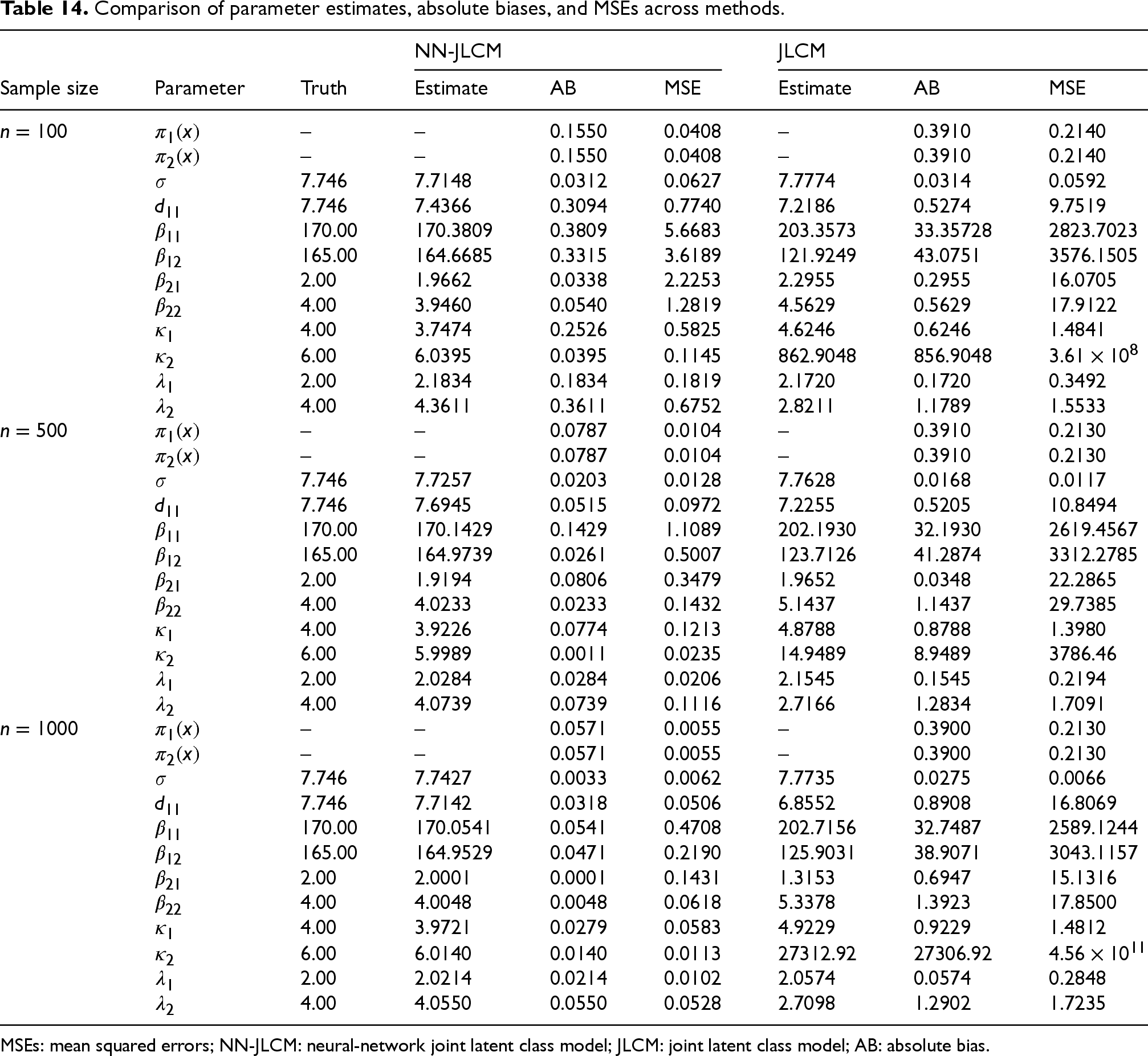
Comparison of parameter estimates, absolute biases, and MSEs across methods.
MSEs: mean squared errors; NN-JLCM: neural-network joint latent class model; JLCM: joint latent class model; AB: absolute bias.
In addition, the mixing proportion bias is larger here for JLCM at around 0.39 in comparison with 0.28 under the same mixing proportion structure in Scenario I. This shows that the logistic class-membership model is structurally unable to recover the true mixing proportions, which are non-monotonic functions, and the bias is compounded when cluster overlap is substantial. The NN-JLCM, by contrast, reduces mixing proportion bias from 0.155 at
Table 15 reports the goodness-of-fit and score test statistics. The NN-JLCM achieves substantially lower CE compared to the JLCM, indicating that the JLCM assigns subjects to classes at little better than chance when clusters overlap. This misclassification propagates to all predictive metrics. The JLCM produces in-sample longitudinal MSE values in the thousands, whereas the NN-JLCM achieves reasonable MSE scores. The IBSs follow a similar pattern, with the NN-JLCM yielding lower values both in-sample and out-of-sample.
Comparison of goodness-of-fit and score test metrics across methods.
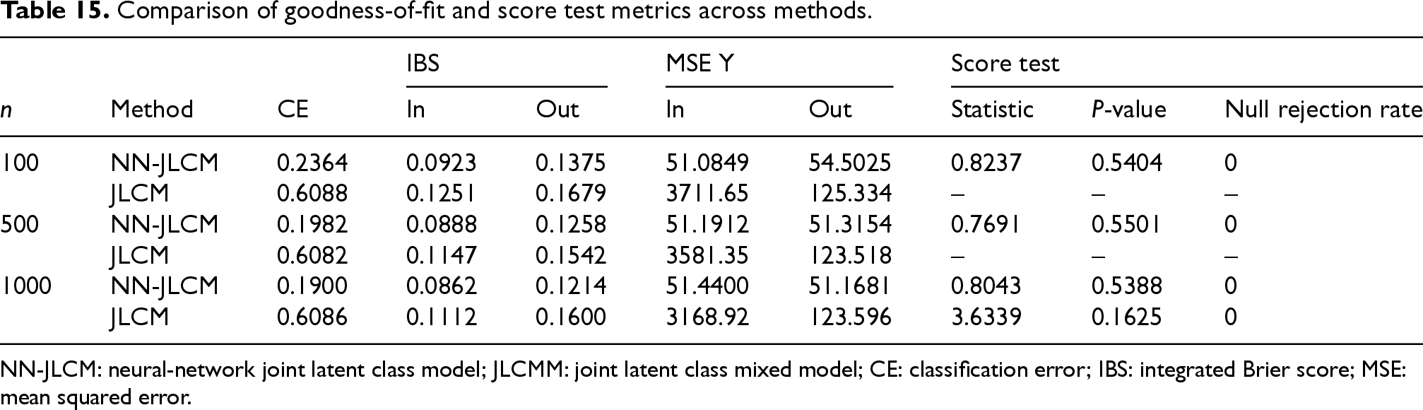
NN-JLCM: neural-network joint latent class model; JLCMM: joint latent class mixed model; CE: classification error; IBS: integrated Brier score; MSE: mean squared error.
The score test for conditional independence fails to reject the null for the NN-JLCM at all sample sizes (statistic
To investigate NN-JLCM’s ability to distinguish between data which conforms to the assumptions of conditional independence, we consider a mirrored approach. Here, data from an SREM is generated, and the various competing models are fit, and then data from a
Further, where the score test is not appropriate, such as the SREM, the Wald test of the association parameter
Generating from an SREM
The settings of this synthetic data analysis are inspired by the primary biliary cholangitis (PBC) dataset from the Mayo Clinic, which has been extensively used in survival analysis literature. 51 The PBC dataset contains longitudinal measurements of serum bilirubin, a biomarker indicative of liver function, alongside time-to-event outcomes for patients with PBC.
We generate data from an SREM to evaluate the score test of conditional independence under a known violation of the JLCM assumption. We briefly discuss the SREM parameterization here but interested readers are directed to Rizopoulos
7
and Papageorgiou et al.
12
for more information. The longitudinal process follows a linear mixed-effects model


The survival process is specified as a Weibull proportional hazards model with the hazard function for subject 
The NN-JLCM and JLCM specifications are the same for the longitudinal and survival submodels with
Results
Table 16 presents the goodness-of-fit statistics for the NN-JLCM, JLCMM, SREM, and JLCT under the SREM DGP. As expected, the SREM consistently achieves the lowest IBS values across all sample sizes, since the fitted model coincides with the true data-generating mechanism. The NN-JLCM and JLCMM yield comparable in-sample IBS values to the SREM, though both exhibit slightly higher out-of-sample IBS, with the JLCMM producing marginally larger values than the NN-JLCM. The JLCT exhibits the poorest predictive performance, with IBS values approximately double those of the other models and substantially inflated MSE values, reflecting the limitations of the tree-based partitioning approach in capturing the smooth, continuous heterogeneity induced by the shared random effects structure. The most notable distinction between the two latent class approaches appears in the longitudinal prediction accuracy. NN-JLCM achieves MSE values matching the SREM, whereas the JLCMM yields substantially inflated MSE values ranging from 5.10 to 6.85. This discrepancy reflects the greater flexibility of the neural network-based mixing proportions in capturing the class-membership structure, which in turn improves the allocation of subjects to their correct longitudinal trajectories.
Goodness-of-fit statistics across sample sizes (SREM DGP,
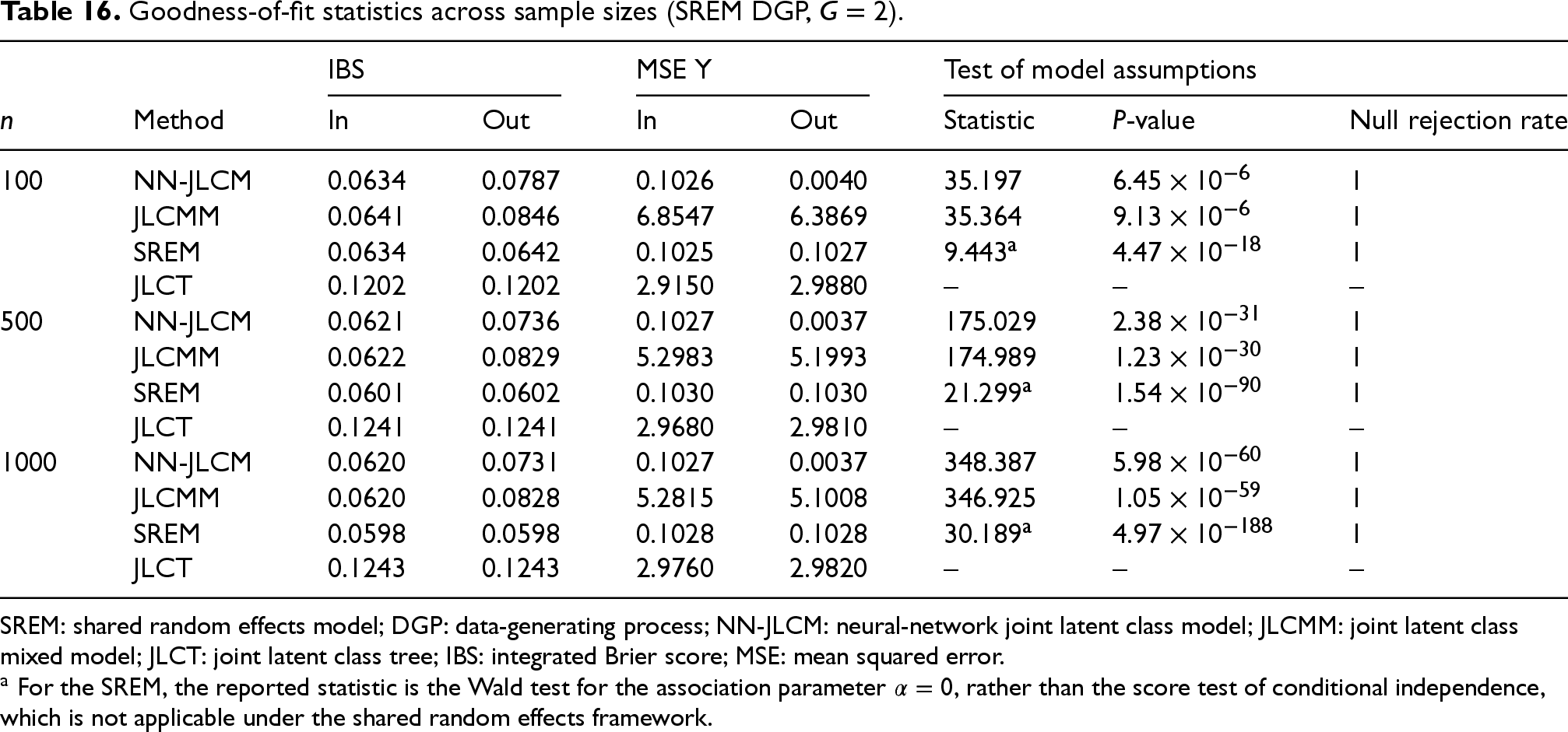
SREM: shared random effects model; DGP: data-generating process; NN-JLCM: neural-network joint latent class model; JLCMM: joint latent class mixed model; JLCT: joint latent class tree; IBS: integrated Brier score; MSE: mean squared error.
The score test of conditional independence correctly rejects the null hypothesis for both the NN-JLCM and JLCMM at all sample sizes, with test statistics increasing proportionally with
The settings of this simulation scenario are also inspired by the PBC dataset.
51
We assume that the true survival times 
We assume that the right-censoring times
To simulate the longitudinal profiles reflecting serum bilirubin trajectories, we consider a class-specific linear mixed-effects model with random intercept and random slope


The class-specific fixed effects are organized into vectors 
To investigate the performance of the methods under non-standard mixing proportion specifications, we adopt a functional form for the class-membership probabilities inspired by the following equation
20
:

We consider three sample sizes:
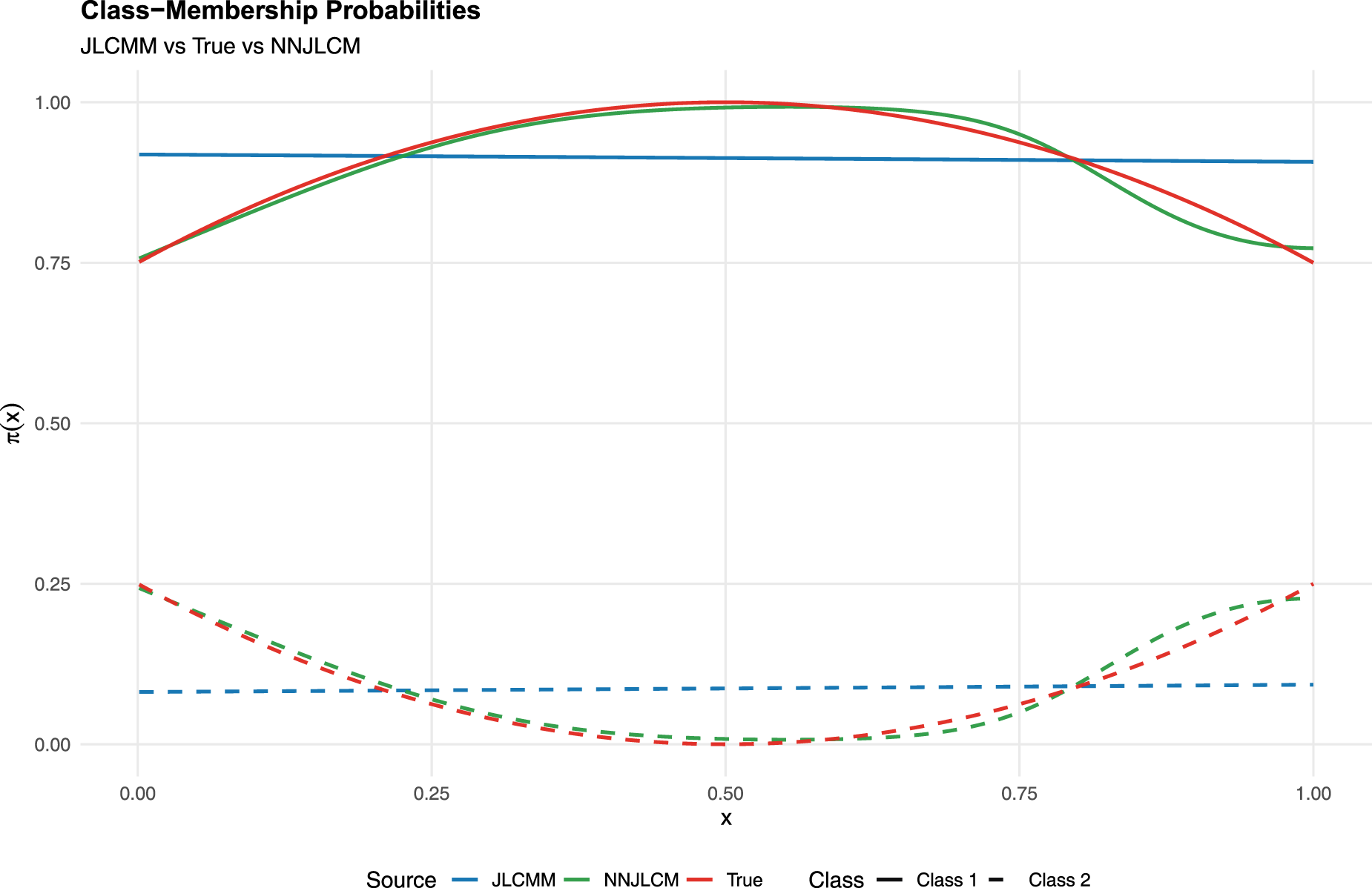
Mixing proportion comparisons for the two-component model under study.
Comparison of goodness-of-fit metrics across methods.
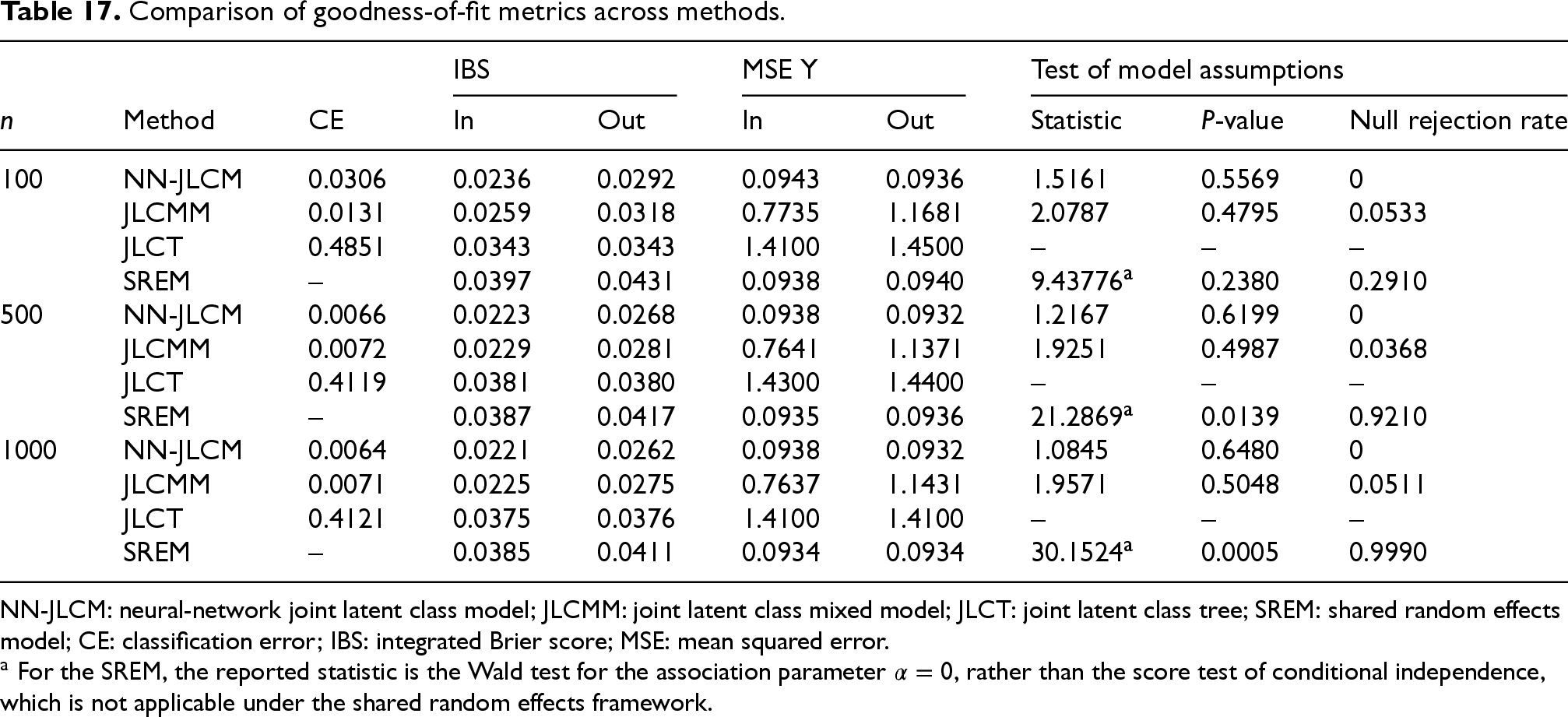
NN-JLCM: neural-network joint latent class model; JLCMM: joint latent class mixed model; JLCT: joint latent class tree; SREM: shared random effects model; CE: classification error; IBS: integrated Brier score; MSE: mean squared error.
Results
The comparison between the four models is revealed in Table 17. In terms of goodness-of-fit, NN-JLCM consistently achieves the lowest in-sample and out-of-sample IBS across all sample sizes, with JLCM producing comparable but slightly higher values, whereas JLCT and SREM lag noticeably behind. The MSE of the longitudinal outcome shows that NN-JLCM and SREM yield nearly identical and substantially lower MSE values, while JLCM produces considerably inflated MSE values, particularly out-of-sample (e.g. 1.1681 at
Regarding the score test, both NN-JLCM and JLCM yield non-significant P-values across all sample sizes, indicating adequate model specification; however, NN-JLCM achieves a null rejection rate of 1.0 in all cases compared to JLCM’s rates around 0.95, suggesting that NN-JLCM more reliably satisfies the distributional assumptions of the score test for this simulation. Interestingly, the SREM’s Wald test for
In this section, we demonstrate the practical use of the proposed model on a real dataset and compare our findings to established models.
PAQUID data description
The PAQUID dataset consists of a random subsample of 500 subjects from the study of a French cohort about dementia and Alzheimer’s incidence rates.
27
The dataset is the benchmark dataset used for both the
Alongside this was the recording of age (age), dementia diagnosis status, dem, and age at dementia agedem. Baseline covariates recorded at enrolment of the cohort are education (CEP), sex (male), and age at enrolment (age_init). MMSE tends to be very skewed in terms of distribution, so the variable is normalized when used in analysis in joint modelling. Age is also replaced with age_65, which is determined by
We plotted the Kaplan-Meier survival curve in Figure 7 along with the risk table. Based on the data, 26% of individuals were diagnosed with dementia at the end of the study. Conversely, there is a very high rate of censoring in the dataset, with a large number of censored times occurring between
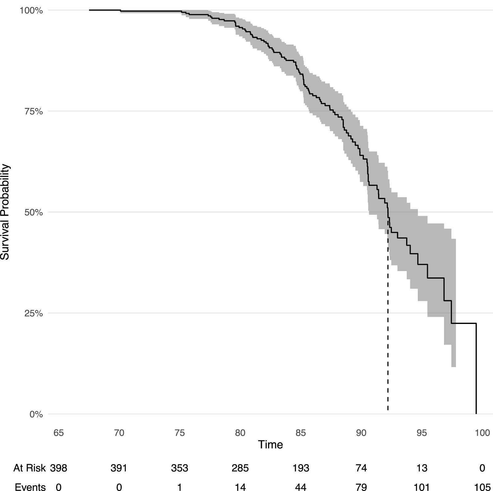
Kaplan-Meier survival curve for the PAQUID dataset.
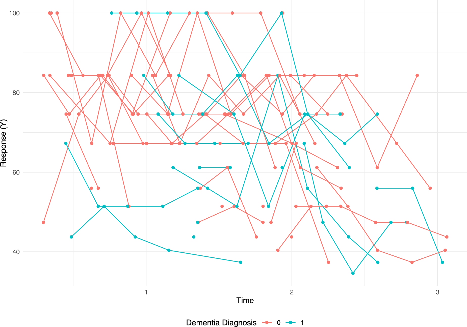
Trajectories for the normalized mini-mental state examination (MMSE) of 50 randomly sampled subjects from the PAQUID study.
Additionally, we plotted the trajectories of the normalized MMSE scores for the PAQUID dataset, where highlighted individuals correspond to a dementia diagnosis (0 indicating no diagnosis and 1 indicating diagnosis). There is not really a clear separation in the trajectories that distinguishes patients with and without dementia for this score, which may suggest the heterogeneity in the population is not directly distinguishable from the plot of the longitudinal profiles (Figure 8).
We consider an 80:20 training-testing split to consider both in-sample and out-of-sample performance of all the models considered. For the class-membership covariates for JLCM, NN-JLCM and JLCT model, we let
Model comparison results.
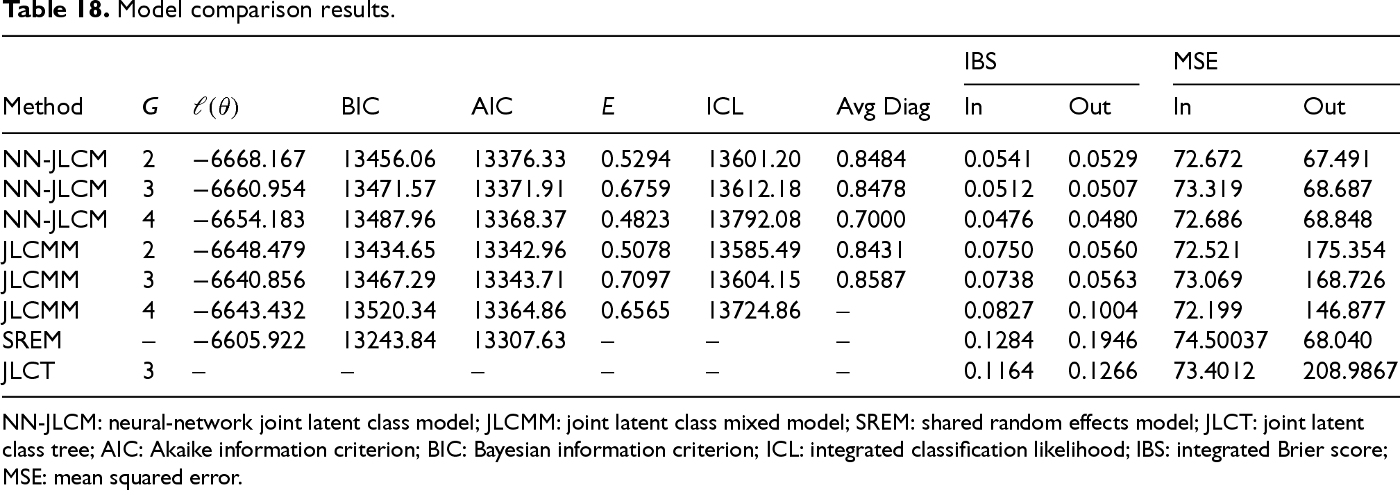
Model comparison results.
NN-JLCM: neural-network joint latent class model; JLCMM: joint latent class mixed model; SREM: shared random effects model; JLCT: joint latent class tree; AIC: Akaike information criterion; BIC: Bayesian information criterion; ICL: integrated classification likelihood; IBS: integrated Brier score; MSE: mean squared error.
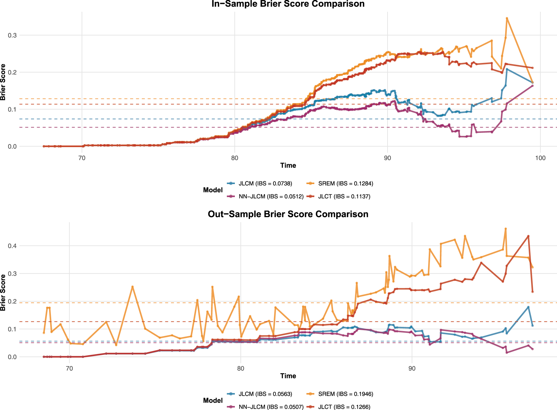
Comparison of Brier scores of survival submodels with integrated Brier score (IBS) indicated in dashes.
We present the performance metrics of the models assessed in Table 18. Again, to determine the ideal number of clusters, we must consider a compromise among a collection of metrics, as it is not so straightforward. If we consider the BIC and ICLs only (i.e. just the information criteria), the ideal model is a
Moving to the classification abilities of the models, the models yielding the best entropy values and the highest average diagonal responsibilities (in the columns entropy and Avg. Diag., respectively) are the three-component models. The probabilities are not computed for the four-class model for JLCMM, as it could not converge after 250 iterations. This also implies the score test could not be computed for that model. Finally, if we consider the predictive abilities of the models, where we can also compare with the JLCT model and the SREM, we can see that the model with the best survival and longitudinal predictive ability for NN-JLCM is one with
In the classical JLCM, all of the covariates in the multinomial logit for class membership were statistically insignificant (not reported), which would suggest that the linear parametric form does not capture the drivers of latent class assignment in this dataset. This is an issue as it effectively limits the JLCM to estimating constant class probabilities.
The NN-JLCM relaxes the linearity restriction and allows for nonlinear mappings from covariates to class probabilities. The results from Table 18 confirm that this additional flexibility improves both the longitudinal and survival predictions. The NN-JLCM showed improvements for both the out-of-sample and in-sample IBS, relative to all other models. To evaluate the goodness-of-fit of our selected models, the BSs were plotted for the entire range of event times in Figure 9. We can see that the BS for every model is about the same until
In summary, the evidence from the PAQUID dataset suggests that the NN-JLCM provides more accurate predictions, clearer class separation, and more robust generalization. The classical JLCM, by contrast, was hindered by the lack of significance in the multinomial covariates for class membership, highlighting the benefits of using a neural network to model mixing proportions.
Conclusion and discussion
In this article, we proposed a NN-JLCM for modelling univariate longitudinal and time-to-event data using an EM-type algorithm to estimate the parameters by maximum likelihood. Extensive simulation studies under varying sample sizes and censoring rates confirmed the competitiveness and robustness of the new method in estimating the survival and longitudinal submodels. Further, simulations in Section 3 showed that if the true class-membership model does not conform to the assumptions of the traditional logistic regression model this can lead to severe biases in predicted survival and longitudinal times as well as poor class discrimination and class-predictions.
Additional studies of finite sample properties in Section 4 considered the efficacy of traditional metrics for latent class selection, a simulation showcasing performance under cluster overlap, and a synthetic data analysis, firstly, considering the effect of generating from an SREM and evaluating the NN-JLCM, JLCMM and the JLCT methods alongside the SREM, and then secondly considering the effect of generating from our proposed model and evaluating all the above competing methods. The purpose of this is to observe NN-JLCM’s behaviour when generating from data which does not conform to the assumptions of conditional independence and vice versa, evaluated through the lens of the score test of conditional independence.
The additional simulations provided useful insights, in that the information criteria and classification metrics under the assumption of a valid score test, adequately predict the true latent class when the class-membership model veers away from the assumptions of the logistic regression model. Further, cluster overlap has mild effects on the performance of NN-JLCM, with a higher CE relative to situations with better class separation. Finally, the synthetic data analysis simulation showed that NN-JLCM behaves as expected when the DGP comes from an SREM, providing an adequate fit in terms of IBS and MSE (comparable to JLCMM) but rejecting the assumption of conditional independence entirely under such a DGP. Similarly, when the DGP conforms to a JLCM, the assumption of conditional independence is held by both NN-JLCM and JLCM.
The application to the PAQUID dataset showcased that while the JLCMM provided an adequate fit in terms of parameters and predictions, the covariates of the multinomial regression were all insignificant and the NN-JLCM still outperformed the JLCM in survival predictions. Additionally, the JLCT model and SREMs were also considered; however, their performance was worse than either JLCM and NN-JLCM. Interestingly, Zhang and Simonoff 17 performed a similar application to the one presented in this article; however, the authors considered a 10-fold cross-validation and evaluated the models only on test data from the cross-validation. Even so, the IBS and MSEs reported here suggest even better performance than what JLCT could achieve. The performance of the SREM is roughly in line with what was observed by Zhang and Simonoff, 17 but to truly confirm this, a cross-validation of NN-JLCM could be investigated on a number of datasets to compare with JLCT.
One of the limitations of the proposed model is that by using a neural network in the class-membership model, we inherently lose explainability and ease of interpretation. Since we use an EM-type algorithm to estimate the parameters, convergence could be slow relative to the Marquardt algorithm implemented in
From here, a potential avenue of future work that could be considered is extensions to multivariate longitudinal data and multivariate time-to-event data. Additionally, the use of semi-parametric specifications for the baseline hazard function could be considered, as well as extensions to other types of longitudinal outcomes such as binary and count data.
Supplemental Material
sj-pdf-1-smm-10.1177_09622802261465334 - Supplemental material for Deep learning embedded latent class joint modelling of time-to-event and longitudinal data
Supplemental material, sj-pdf-1-smm-10.1177_09622802261465334 for Deep learning embedded latent class joint modelling of time-to-event and longitudinal data by Tristan John Elers Harris, Najmeh Nakhaei Rad and Sphiwe Bonakele Skhosana in Statistical Methods in Medical Research
Footnotes
Acknowledgements
The authors would like to thank the two independent reviewers for their insightful comments and suggestions that have greatly improved the quality of this article.

Funding
The research of the second author is supported in part by the National Research Foundation (NRF) of South Africa, Ref.: RA210106581084, grant No. 150170. The opinions expressed, and the conclusions arrived at, are those of the authors, and are not necessarily to be attributed to the NRF. Additionally, the work reported herein was made possible through funding by the South African Medical Research Council (SAMRC) through its Division of Research Capacity Development under the SAMRC Clinician Researcher Development Programme, with funding received from the National Department of Health. The SAMRC funding was awarded to the first author as part of his PhD funding. The content hereof is the sole responsibility of the authors and does not necessarily represent the official views of the SAMRC.
Declaration of conflicting interest
The authors have no conflicting interests to declare with respect to the research, authorship, and/or publication of this article.
Supplemental material
Supplemental material for this article is available online.
References
Supplementary Material
Please find the following supplemental material available below.
For Open Access articles published under a Creative Commons License, all supplemental material carries the same license as the article it is associated with.
For non-Open Access articles published, all supplemental material carries a non-exclusive license, and permission requests for re-use of supplemental material or any part of supplemental material shall be sent directly to the copyright owner as specified in the copyright notice associated with the article.
