Benchmarking support vector regression against partial least squares regression and artificial neural network: Effect of sample size on model performance

Abstract

It has become easy to obtain multivariate chemical data of high dimensions. However, it may be expensive or time consuming to obtain a large number of samples or to acquire reference measures, so the number of samples available for multivariate calibration modelling may be limited. If data contains nonlinear relationships, nonlinear methods are required for the calibration task. The combination of limited amounts of data of high dimensions and highly flexible nonlinear methods may result in overfitted models which in turn perform badly on new data. Therefore, for real world applications, it is desirable to understand how the sample size affects model prediction performance. For this purpose, we compared partial least squares regression, artificial neural network, and support vector regression applied to three real world nonlinear datasets of which two were of high dimensions. We evaluated the effect of calibration sample size (i) on test set performance, including variation in test set performance due to sampling variation and (ii) tested if the cross-validated performance was adequate for assessing the predictive ability. We demonstrated the applicability of artificial neural network and support vector regression for real world data of limited size and showed that support vector regression had advantages over artificial neural network: (i) fewer calibration samples were required to obtain a desired model performance, (ii) support vector regression was less sensitive to sampling variation for small sample sets and (iii) cross-validation was an approximately unbiased option for evaluating the true support vector regression model performance even for small sample sets.

Keywords

Sample size prediction performance cross-validation high dimensional data artificial neural network partial least squares regression support vector regresssion near infrared

Introduction

During the last decades, there has been an increase in sophisticated chemical analytical methods generating data with a very high number of variables. Multivariate modelling methods are usually required to relate such data to the desired biological, chemical or physical property. In particular, partial least squares regression (PLS) is widely applied for chemical data analysis. However, assuming linearity sometimes leads to suboptimal models, because the relationships modelled are indeed nonlinear. Near infrared (NIR) spectra and quantitative structure–activity relationship (QSAR) data are examples of data often exhibiting various types of nonlinearities. Changes in the physical and chemical constitution of a sample, such as temperature and pH, cause spectral shifts or in other ways non-fulfilment of Beer’s law.^1–3 In the case of QSAR data, the descriptors may be intrinsically nonlinearly related to the property of interest.

Nonlinear methods are not widely applied for modelling of chemical data. The reasons for avoiding these methods are many and include too little knowledge on (i) which method to choose, (ii) how to optimize the model including selection of meta-parameters, (iii) sample size requirement, (iv) how to deal with noise and outliers and (v) computer power requirement. Dogmatic perceptions such as common practice and possibly faulty views of nonlinear methods being very difficult to deal with obstruct the dissemination of these methods. In order to gain wider currency, information on how to build and interpret nonlinear models should be easily available.

In this paper, we address the prediction performance of calibration models PLS, artificial neural network (ANN) and support vector regression (SVR) under different calibration sample sizes. This is important because although it has become easy to measure a high number of variables for many types of analyses, it may still be expensive and time consuming to obtain a large number of samples or to acquire adequate reference measures for model development. Therefore, for real world applications, it is desirable to understand how the sample size affects model prediction performance.

Nonlinear modelling of limited amounts of data is particular challenging when data are high dimensional and this is partly due to the curse of dimensionality where model flexibility increases with increasing data dimensionality. In general, a more flexible model needs more calibration data to determine its parameters accurately. Nonlinear methods add to the curse of dimensionality, since they intrinsically offer more flexibility than linear methods do, simply because they can fit more complicated relations.

SVR is a nonlinear method which is characterized by high generalization ability.⁴ SVR and support vector machines (SVM) for classification entered the chemical literature around 2000.^5–9 Since then, SVR has gained increasing interest within chemometrics,^10–12 but its dissemination in real world applications is still limited compared to ANN,^10,13–15 where the latter has been a tool for analysis of chemical data since late 1980s.¹⁶ ANN is generally considered to require a very large number of calibration samples to avoid overfitting.^17–19 Numerous papers compared the performance of SVR and ANN on various types of chemical data, mostly to the benefit of SVR.^11,19,20 However, only few examples of a systematic investigation of the impact of calibration sample size on prediction performance exist for regression^21,22 and for classification.^23,24 All obtained similar results, namely that SVM and SVR performed better than ANN for all sample sizes but especially for small sample sizes.

None of these previously examined datasets were of very high dimensions. This paper reports a systematic study of the effect of sample size on model performance for high dimensional chemical data. For this purpose, PLS, ANN and SVR were applied to (i) a dataset of NIR spectra measured at 450 wavelengths, predicting sucrose. To further exemplify and understand the performance, the models were also investigated on (ii) a QSAR dataset containing 150 2D descriptors, predicting melting point, and (iii) a dataset containing eight quantitative attributes of concrete, predicting compressive strength. The obtained models were evaluated as follows: (i) model performance was evaluated as root mean squared error of an independent test set (RMSEP) and the effect of sampling variation on model performance was evaluated as the variation in RMSEP as a result of models built on 30 realizations of a calibration dataset of a defined number of samples (n). Moreover, (ii) the adequateness of using cross-validation for assessing predictive ability was evaluated as RMSEP relative to the root mean squared error of cross-validation (RMSECV): percentage of (RMSEP–RMSECV)/RMSECV which we named cross-validation optimism (CV optimism). A low CV optimism would reveal RMSECV as a reliable measure of the true model performance and hence could be used for model validation. This in turn could reduce the number of samples required for a calibration task, since setting aside samples for an independent test set could be avoided.

Theory

Support vector regression

The main characteristics of SVR are outlined in Table 1. The basis of SVR is multiple linear regression which can be expressed as y = f(x) + ɛ where

\begin{matrix} f (x) = w^{T} x + b \end{matrix}

(1)

where the observation vector x and reference value y are the independent and dependent variables, respectively, and w and b the regression vector and offset, respectively. The equation holds for every observation. SVR seeks a solution that has at most ɛ deviation, in absolute terms, from the observed reference value for all observations, and introduces the so-called ɛ-insensitive loss function to penalize training errors larger than ɛ²⁵

\begin{matrix} L (y) {\begin{matrix} 0 & if | y - f (x) | < ɛ \\ | y - f (x) | - ɛ & otherwise \end{matrix} \end{matrix}

(2)

Table 1.

Overview of main characteristics of PLS, ANN and SVR.

	PLS	ANN	SVR
Method	Linear	Nonlinear	Nonlinear
Loss on training error	Least squares	Least squares	Epsilon insensitive
Model complexity mainly controlled by	Selection of latent variables	Selection of nodes in input and hidden layers	Minimization of w′w
Meta-parameters	Number of latent variables	Number of layers, number of nodes in each layer.	Kernel parameter, C and ɛ
Additional parameters	None	Transfer function, initial values of weights, optimisation cycles.	Type of kernel
Solution	Unique	Local minima exist	Unique
Strategy for handling high dimensional data	Compression of data by latent variables	Compression of data by latent variables	Input data presented as inner products

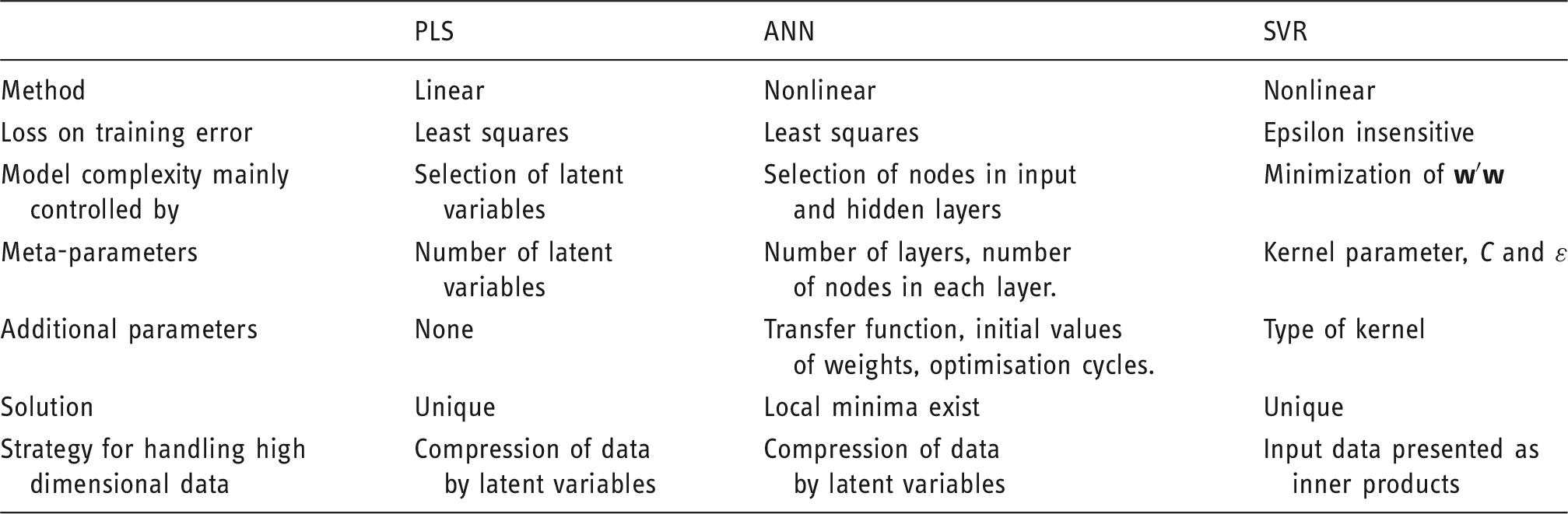
ANN: artificial neural network; PLS: partial least squares regression; SVR: support vector regression.

Further, in order to obtain a model which generalizes beyond the training data, a penalty is put on large regression coefficients through a penalty on the length of w, and a user-defined parameter, C, trades-off focus on generalization and training error. The SVR problem can be formulated as a convex optimization problem with constraints²⁵

\begin{matrix} {min}_{w, ξ} \frac{1}{2} w^{T} w + C \sum_{i = 1}^{n} (ξ_{i} + ξ_{i}^{*}) \end{matrix}

\begin{matrix} subject to {\begin{matrix} y_{i} - w^{T} x_{i} - b \leq ɛ + ξ_{i} \\ w^{T} x_{i} + b - y_{i} \leq ɛ + ξ_{i}^{*} \\ ɛ, ξ_{i}^{*}, ξ_{i} \geq 0 \end{matrix} \end{matrix}

(3)

The slack variables ξ_i, ξ_i* are introduced for the situations where f(x _i ) differs by more than ɛ above (ξ_i) or below(ξ_i*) from the observed reference value (i = 1,…, n). Equation (3) is a standard quadratic programming problem, which can be reformulated into a dual problem formalism and solved using Lagrange multipliers: α_i and α_i* (0 ≤ α_i, α_i* ≤ C). Hence the solution is expressed in terms of the Lagrange multipliers rather than the regression vector w from equation (1) ²⁵

\begin{matrix} f (x) = \sum_{i = 1}^{n} (α_{i} - α_{i}^{*}) 〈 x_{i}, x 〉 + b \end{matrix}

(4)

Here $〈 x_{i}, x 〉$ denotes the inner product of the training object x _i and a new sample x, to be predicted. The entry of data in the form of inner products in equation (4) is important because: (i) the dimensionality of the training vectors does not appear in the problem to be solved and (ii) extensions of this linear approach to nonlinear regression can be made easily using so-called kernel functions. The strategy of SVR is to stick with linear functions, which are simple and hence easy to estimate, but create additional flexibility by working in a high dimensional feature space. When kernel functions K(x _i ,x _j ) meet certain conditions,^7,26 they implicitly determine a nonlinear mapping x _i → Ф(x _i ) as well as the corresponding inner product (Ф(x _i ), Ф(x _j )). From equation (4) it follows that replacing the inner product $x_{i}, x$ with the inner product in the feature space (Ф(x _i ), Ф(x _j )) leads to the solution for the nonlinear situation

\begin{matrix} f (x) = \sum_{i = 1}^{n} (α_{i} - α_{i}^{*}) K (x_{i}, x) + b \end{matrix}

(5)

One of the most widely used kernel functions is the radial basis function (RBF) kernel⁷

K (x_{i}, x_{j}) = \exp (- \frac{x_{i} - x_{j}_{2}^{2}}{2 σ^{2}})

(6)

The kernel width, σ, controls the size of a neighbourhood around a support vector where it influences predictions of new samples.

The three meta-parameters C, ɛ and σ must be selected by the user prior to model estimation. As they jointly influence model generalisation, they should be optimized simultaneously.

PLS and ANN

PLS and ANN will not be described here, but instead the reader is referred to the literature.^27–29 The main features, though, are outlined in Table 1 along with the characteristics of SVR. The linearity of PLS imposes limitations on the model but PLS only requires determination of a single meta-parameter, namely the number of latent variables. It is deterministic and the solution is unique under most circumstances. The nonlinear ANN requires optimization of a number of meta-parameters including selection of transfer function(s) and number of optimization cycles. Further, the ANN solution is not unique and depends on initialization. Compression of data e.g. by PLS prior to modelling is often used to bound the model flexibility.

Data descriptions and methods

Three datasets containing nonlinearities were investigated in order to assess the performance of PLS (standard linear method), ANN (standard nonlinear method) and SVR (alternative nonlinear method) under different amounts of calibration data. The main characteristics of the datasets are presented in Table 2. The term ‘n training’ refers to the number of samples in the training set and ‘n test’ refers to the number of samples in the test set.

Table 2.

Overview of main characteristics of the three datasets.

Dataset	n training	n test	Variables	Response	Range of response	References
NIR	1189	608	450	Sucrose	12.9–78% w/w	[30]
QSAR	9963	2626	150	Melting point	−157℃–389℃	[33]
Concrete	847	171	8^a	Compressive strength	2.3–82.6 MPa	[34]

NIR: near infrared; QSAR: quantitative structure–activity relationship.

Quantitative attributes of concrete.

NIR spectra from a sugar factory for prediction of sucrose

The main dataset was from a sugar factory and contained NIR measurements from four process steps aimed for prediction of sucrose.³⁰ The dataset contained nonlinear effects due to changes in the physical and chemical constitution of the process stream during production. A total of 1800 samples were measured at 400–1890 nm with an increment of 2 nm. Models were built on 450 selected variables.³⁰ Sucrose, the reference variable was measured in weight percentage. The dataset was split into calibration (66%) and test (33%) set using the so-called onion method as implemented in PLS_Toolbox version 7.9 (Eigenvector Research, Inc. Wenatchee, WA).³¹ The splitting was manually evaluated in order to ensure that the two sets seemed to be similarly distributed.

QSAR data for prediction of melting points

Prediction of melting points are important for various applications such as assessment of hazardousness of chemical compounds in REACH^a or in the medicinal and environmental chemistry for estimating solubility.³² Prediction of melting point from QSAR data is known to be difficult, as indicated by high prediction errors of previously reported models (RMSEP >31℃).^32,33 The present QSAR dataset has a total of 12,589 compounds with 150 two-dimensional descriptors and originated from several different databases.³³ The dataset was split into calibration and test set similar to the NIR dataset.

Concrete data for prediction of compressive strength

The concrete dataset was included in the study as a third and very different dataset in order to investigate if the sample size dependence was mainly data type dependent or if a more general tendency existed. This dataset was an extended version of the dataset used by Yeh.³⁴ It consisted of eight quantitative attributes of manufactured concrete for a total of 1030 samples for prediction of the compressive strength of high performance concrete. According to Yeh³⁴ the compressive strength of concrete was a highly nonlinear function of age and ingredients. The eight attributes showed very little linear correlation to the compressive strength. The dataset was split into calibration (83%) and test set (17%) using the onion method.

Study design

The following procedure was applied to all three datasets: New datasets of decreasing number of calibration samples were obtained by sampling 50% of the previous calibration set. This was done until the obtained training set reached a size of approximately 18 samples. Thirty series of such dataset realizations were generated.

For generalisation of the results in this study it was assumed that the sampling of calibration data was drawn from an infinite pool of samples, which directly implied independence between calibration data sets. However, the data were real and consequently from a finite pool of samples, which introduced dependency between calibration data sets. For the calibration sample sizes close to the size of the total sample pool this entailed that the variation in RMSEP was biased downwards due to the calibration models being constructed from data with overlapping samples. This leads to a 40% and 15% underestimation of the variation in RMSEP of models based on 50% and 25% of the total sample pool, respectively. For the remaining sample sizes, the effect was negligible. Moreover, it did not affect the comparison between the different methods, which is why we have not corrected the results in this regard.

Methods and software

The NIR data were corrected using a standard normal variate (SNV) followed by ordinary mean centring of the columns of the data matrix. The QSAR and concrete datasets contained discrete x-variables and hence autoscaling was applied. All reference variables were mean centred. For each data type, strongly outlying samples were removed from an initial PLS model built on all calibration samples. Automated selection of meta-parameters was applied to all methods selecting the setting with the smallest error from a 10-fold cross-validation (RMSECV). Models were validated by RMSEP of the independent test set. Furthermore, CV optimism was measured as the percentage (pct.) of (RMSEP–RMSECV)/RMSECV.

PLS

One to 20 latent variables were investigated for the minimum RMSECV in case of the NIR and QSAR data and a maximum of eight latent variables were investigated in case of the concrete dataset.

ANN

A feed forward, backpropagation neural network was used. To prevent overfitting, it comprised a single hidden layer and data were compressed by PLS in order to reduce the number of nodes in the input layer. A grid-search was used to select the optimal number of latent variables in the PLS model and optimal number of nodes in the hidden layer. The maximum values of the meta-parameters were: NIR data: nine latent variables and nine nodes, QSAR data: six latent variables and eight nodes, concrete data: eight latent variables and 12 nodes. A maximum of 20 learning cycles were used in the model optimization, and the actual number of cycles, number of latent variables and nodes was selected by the minimum of RMSECV. The adopted ANN algorithm used random initialization of the weights and there was no weight decay for the single hidden layer.

SVR: Grid search was applied for selection of C, ɛ and the σ parameter in the RBF kernel. All three meta-parameters were searched in a log2 scale and selected by cross-validation.

Calculations were made in MATLAB R2014a (The MathWorks, Inc., Natick, MA) and PLS_Toolbox version 7.9 (Eigenvector Research, Inc. Wenatchee, WA).

Results and discussion

NIR data

Figure 1(a) shows box plots of the test set error of the models built on the NIR spectra. All modelling methods showed similar influence of sample size on model performance: The test set error increased very little when the number of calibration samples was reduced from 1134 to 143. A further reduction in sample size lead to a steady increase in test set error for PLS and SVR and an exponential increase for ANN. However, the increases were moderate in general.

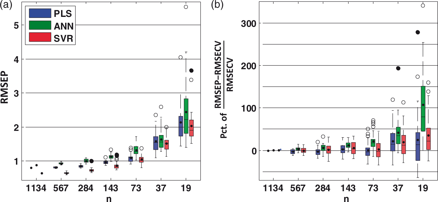
The almost constant performance of all methods for large n suggested that all calibration models had approached their minimal model error. The RMSEP of SVR was close to the reference uncertainty of 0.5³⁰ indicating that SVR had sufficient flexibility to model the true relationship in the data. The higher error of PLS was likely due to its intrinsic limitations in modelling nonlinearities.

SVR showed the smallest median RMSEP in the entire range of calibration sample sizes. For n ≥ 143 samples, one could be almost certain to obtain a SVR model that performed better than a corresponding PLS or ANN model as shown by no or very little overlap in the distribution of the obtained test set errors of the methods. For the smallest sample sizes, test set error was similar for all methods except ANN which showed a sudden increase in RMSEP variation for 19 calibration samples. Yet, ANN performed surprisingly well even for small sample sizes.

It was unexpected that PLS would perform better than ANN for large sample sizes, in part because of the automated selection of PLS latent variables, which selected a, from a chemical viewpoint, unrealistically high numbers of variables. E.g. all models based on 567 calibration samples contained the maximum of 20 latent variables.^b However, these models that contained a high number of latent variables did perform well.

Moderate increases in RMSEP variability were observed for all methods when the number of calibration samples was reduced, demonstrating that one should be increasingly concerned that the calibration samples indeed represented future samples well when the number of calibration samples was limited. This was especially an issue for ANN models built on 19 samples.

PLS and SVR did not show much CV optimism in general until n ≤ 37 samples and the variability only increased slowly, illustrating highly reliable RMSECV estimates (Figure 1(b)). In contrast, ANN displayed a consistently positive central distribution (CD – the interval from the lower 25% to the upper 75% quartile depicted as the box in the box plot) of the CV optimism, which was slowly growing until 37 calibration samples. After that, the CV optimism, as well as the RMSEP, increased significantly, pointing at a breakdown in ANN generalization ability.

QSAR data

Figure 2(a) outlines the test set performance of models built on the QSAR data. Generally, the test set errors were high which agreed with previously reported models.^32,33,35 Possibly the high error derived from a deficiency in the descriptors for explaining the melting point.³⁵ Moderate overall reduction in ANN and SVR model performance was observed, as the median RMSEP increased by 75% for ANN and 81% for SVR when the number of calibration samples was reduced from 9964 to 20. In contrast, the median RMSEP of PLS increased by 537%.

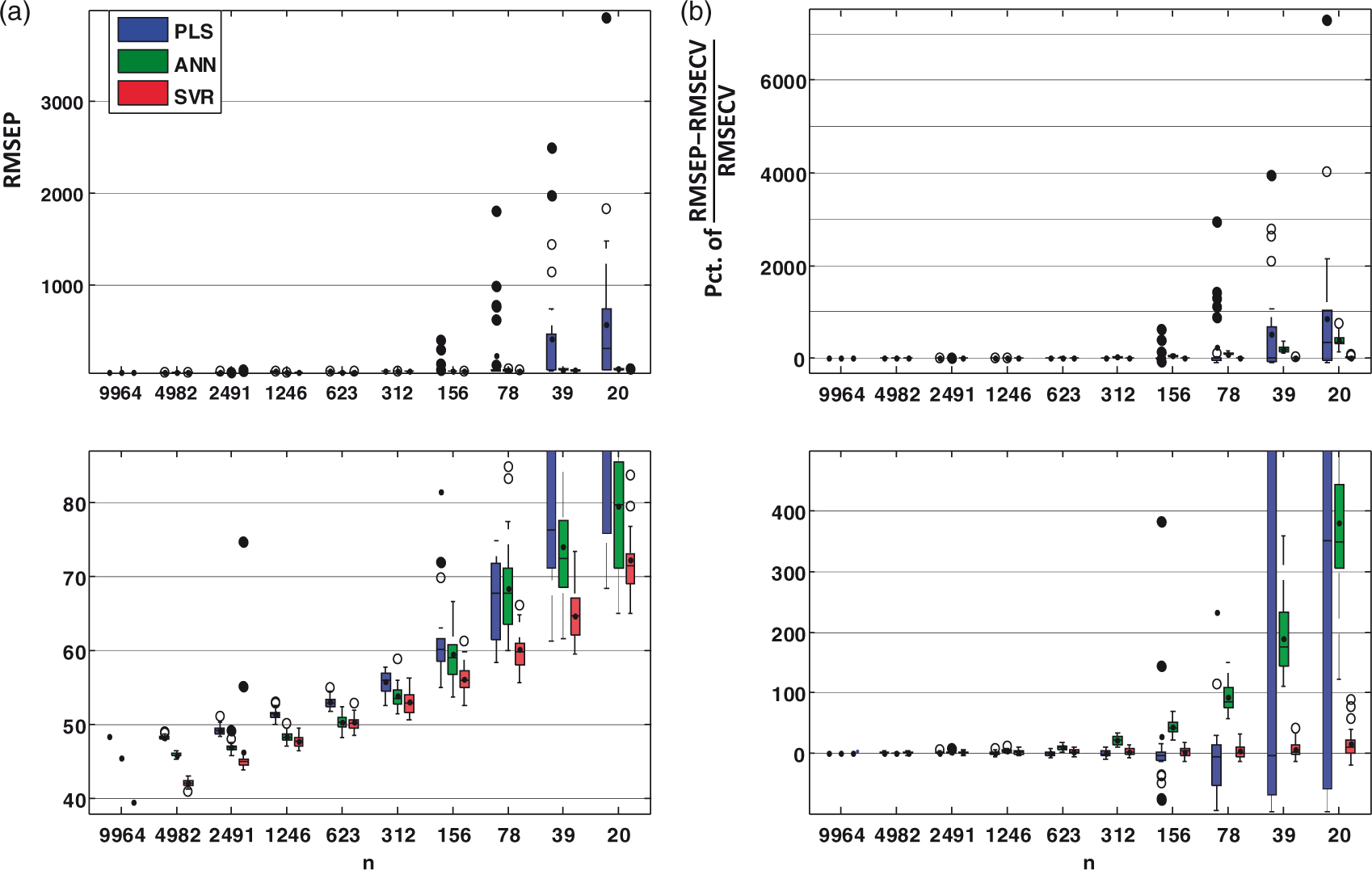
SVR performed significantly better than PLS and ANN. Indeed, there was no overlap of PLS and SVR CD for any calibration sample size. There was no overlap between ANN and SVR CD for five sample sizes, but they performed similarly for 623 and 312 calibration samples.

The median RMSEP of SVR models increased steadily throughout the entire range of calibration samples tested. PLS and ANN median RMSEP were fairly flat for large n but showed a growth increase for n = 1246 to 20, with faster growth for PLS than for ANN. Hence, SVR was less affected by small calibration samples sizes than PLS and ANN. The levelling off in PLS and ANN RMSEP for large n indicated that they approached the maximum capacity of the methods for modelling the data. The levelling off appeared for similar sample sizes, but ANN obtained lower test set error than PLS, indicating its better ability for modelling nonlinear relationships. On the other hand, the steady improvement in SVR RMSEP indicated that SVR could continue to improve significantly if built on more calibration samples than included in this study.

SVR was highly robust against sampling variation as indicated by the generally low RMSEP variation as well as its limited increase for decreasing number of calibration samples. PLS was not affected much by sampling variation until n = 156, at which point some models obtained test set errors several times larger than the median error. Reducing the number of calibration samples further led to extreme test set performances for an increasing number of models. A similar pattern was observed for CV optimism of the PLS models (Figure 2(b)). These patterns were in stark contrast to ANN and SVR, although they were all presented with the exact same dataset realizations. Therefore, these observations pointed at PLS being insufficient in modelling the true structure in the data, likely due to linearity imposing limitations upon model flexibility. In combination with the high level of PLS model error in general and low sample size, it made PLS highly sensitive to sampling variability. The nonlinear methods, on the other hand, apparently matched the data structure better and had lower error level, so they could more accurately aim for the relevant variation in data regardless of the specific data representation. However, ANN was more sensitive than SVR to sampling variation revealed by consistently higher variation in test set error.

Figure 2(b) shows a significant increase in ANN CV optimism reaching 380% on average (median CV optimism) for n = 20 samples. This indicated that the models fitted the calibration data very (too) well and hence generalized poorly. However, the test set performance was not extreme compared to SVR. Hence, our results demonstrated that it was possible to obtain fairly well performing ANN models although they overfitted the calibration data. It was crucial, though, to use an independent test set for model validation. The CV optimism of SVR was low for all sample sizes, why RMSECV was a reliable measure of the true model performance even for as little as 20 calibration samples.

Concrete data

SVR and ANN had very overlapping test set error of the concrete dataset in general. However, an increasingly smaller test set error of SVR compared to ANN was observed for n = 53 to 14 samples. Both nonlinear methods continued to improve for high n, whereas PLS started to level off at n = 53. That is, PLS approached its minimum error at a relatively small sample size whereas no indication of a similar approach was observed for ANN and SVR for the sample sizes studied.

Small differences in RMSEP variability between the methods indicated that PLS was least sensitive to sampling variation, which agreed with the expectation that a less flexible model will over fit less and hence be less sensitive to small variations in calibration data.

The concrete models showed CV optimism profiles similar to the NIR models. However, for n = 14, all methods showed similarly CV optimisms, meaning that RMSECV became an equally uncertain measure of model performance (Figure 3(b)).

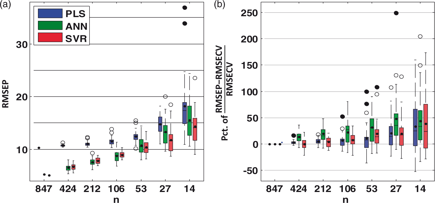
Comparison of the methods across the datasets

Model performance

All methods showed a similar overall performance profile for decreasing amounts of calibration data across data types; the model performance decreased when the amount of calibration data was reduced. For a specific method and specific dataset, the calibration sample size dictated the model performance; an observation supported by classical statistical theory.

In the present study, SVR performed better than PLS and ANN for all sample sizes of all datasets, with only a few exceptions where PLS or ANN performed similar to SVR. Hence, our results demonstrated the high generalization performance of SVR and indicated that it applies to large as well as small sample sizes. For large sample sets it was noteworthy that SVR performed better than the nonlinear alternative, ANN, for two out of three datasets.

PLS was least affected by sample size, except for the QSAR data. But contrary to our expectations, this was due to poor performance on large sample sets only, and not due to good performance on small sample sets. In general, only moderate reduction in test set performance was observed (a factor of three for median RMSEP) when the calibration data were reduced from several thousand samples to approximately 20 samples. This was particularly surprising for ANN, which we expected to display a strong decrease in model performance when sample sizes were reduced. Hence, our results challenge the dogmatic perception of ANN requiring a high number of calibration samples in order to perform well. However, the ANN modelling was not conducted directly on the raw data but on a latent factor compression of those. This indeed bounds the model flexibility and hence the potential for overfitting, and might be more central in this aspect than the ANN model-framework itself.

Cross-validation optimism

When the number of calibration samples is limited, an adequate cross-validation optimism is critical for using RMSECV as a reliable estimate for model validation. In such cases, samples are not required for an independent test set which reduces the number of samples required for model building and validation. However, RMSECV was also used for selecting appropriate meta-parameters so, the RMSECV values can be slightly optimistic. The three calibration methods demonstrated consistent CV optimism profiles across datasets (Figures 1(b), 2(b) and 3(b)), indicating that the effect of sample size on CV optimism follows a certain pattern regardless of the type of data. However, PLS models of the QSAR data (Figure 2(b)) illustrated that exceptions do exist.

SVR obtained equally low CV optimism as PLS, even though RMSECV was used to select three meta-parameters rather than the single parameter for PLS. The negligible CV optimism of the PLS and SVR models implied that the model performance could be evaluated using cross-validation and thus the need for setting aside samples for a test set was avoided. This is especially valuable in practical applications where data are limited due to e.g. cumbersome or expensive sample collection as well as attainment of reference measures.

ANN obtained positive CV optimism in general. This resulted from a more extensive use of the cross-validated error for parameter selection during ANN model building compared to PLS and SVR: selection of meta-parameters as well as deciding the number of learning cycles for ANN parameter estimation was all based on RMSECV. While this extensive use of RMSECV had no implications for large datasets, which held sufficient information to estimate the model parameters accurately, it biased RMSECV downwards for small datasets. However, it had only minor influence on the models, since ANN performance was only a little poorer than the SVR performance for similar calibration data sizes.

As a consequence of the high CV optimism, proper evaluation of ANN model performance required test set validation. This pointed at another disadvantage of ANN: in addition to requirement of a larger calibration sample set in order to obtain model accuracy similar to SVR, it also required samples set aside for evaluating the true model performance.

High dimensional data

Our study revealed a moderate effect of sample size on model performance although two of the three data types were of very high dimensions. The only extreme result was obtained for the linear PLS on the highly complex QSAR dataset and not for the more flexible nonlinear methods, indicating that the combination of high dimensions and high model flexibility, even for small sample sizes, did not radically impair model prediction performance. This may be due to the strategies for data reduction either by latent factor compression (ANN) or application of kernels (SVR), which indeed restrained the curse of dimensionality.

Conclusion

In this paper, we applied PLS, ANN and SVR to three very different datasets containing nonlinearities in order to study the effect of calibration sample size on model prediction performance. The nonlinear methods performed equally well or better than PLS for even small sample sizes and in general only moderate effects of sample size were observed. Hence, our results challenge the dogmatic perception of ANN requiring a high number of calibration samples in order to perform well. SVR obtained consistently low CV optimism and superior model performance which pointed at a high generalization ability, even for small sample sets. Two datasets were of high dimensions, which illustrated that the combination of high dimensions and high model flexibility for even small sample sizes did not radically impair ANN and SVR prediction performance.

We demonstrated the applicability of nonlinear calibration methods for real world applications where the amount of calibration data can be limited. Our results indicated that practitioners have no need to hesitate on using ANN and SVR due to concerns about sample size requirements. Particularly, our results pointed at SVR as a good candidate for real world applications, as it showed a number of advantages over ANN as implemented here: (i) generally it obtained higher accuracies, why fewer calibration samples were required to obtain a desired model performance and (ii) for small calibration datasets, it was less sensitive to sampling variation. However, smaller sample sizes were in general associated with higher variance in RMSEP. Finally (iii) SVR was robust against CV optimism for even relatively small sample sizes, so cross-validation was a realistic option for validation of the true model performance. In a case of limited availability of samples, this would significantly reduce the sample requirement since a test set would not be needed. Additional advantages of SVR are its global solution, its deterministic behaviour and a more straightforward meta-parameter selection although selection of optimal meta-parameters may require substantial computer power and be highly time consuming.

Footnotes

Acknowledgement

The authors acknowledge Daito Togyo Corporation, Japan for providing the process samples.

Declaration of conflicting interests

The author(s) declared no potential conflicts of interest with respect to the research, authorship, and/or publication of this article.

Funding

The author(s) received no financial support for the research, authorship, and/or publication of this article.

Notes

References

Hageman

Westerhuis

Smilde

. Temperature robust multivariate calibration: an overview of methods for dealing with temperature influences on near infrared spectra. J Near Infrared Spectrosc 2005; 13: 53–62.

Miller

. The chemometric space. Sources of non-linearity i near infrared methods. NIR News 1993; 4: 3–5.

Bertran

Blanco

Coello

et al.

Determination of olive oil free fatty acid by Fourier transform infrared spectroscopy. J Am Oil Chemists Soc 1999; 76: 611–616.

Cortes

Vapnik

. Support-vector networks. Machine Learning 1995; 20: 273–297.

Burbridge

Trotter

Buxton

et al.

Drug design by machine learning: support vector machines for pharmaceutical data analysis. Comput Chem 2001; 26: 5–14.

Cai

Liu

et al.

Prediction of protein structural classes by support vector machines. Comput Chem 2002; 26: 293–296.

Belousov

Verzakov

von Frese

. A flexible classification approach with optimal generalisation performance: support vector machines. Chemometr Intell Lab Syst 2002; 64: 15–25.

Bock

Gough

. Predicting protein–protein interactions from primary structure. Bioinformatics 2001; 17: 455–460.

Brown

MPS

Grundy

Lin

et al.

Knowledge-based analysis of microarray gene expression data by using support vector machines. Proc Natl Acad Sci U S A 2000; 97: 262–267.

10.

Nantasenamat

Isarankura-Na-Ayudhya

Naenna

et al.

Prediction of bond dissociation enthalpy of antioxidant phenols by support vector machine. J Mol Graph Modell 2008; 27: 188–196.

11.

Akbari

Buntat

Enzevaee

et al.

Analytical modeling and simulation of I–V characteristics in carbon nanotube based gas sensors using ANN and SVR methods. Chemometr Intell Lab Syst 2014; 137: 173–180.

12.

Chen

Zhang

Ning

et al.

Predicting the anthocyanin content of wine grapes by NIR hyperspectral imaging. Food Chem 2015; 172: 788–793.

13.

Köksal

Batmaz

Testik

. A review of data mining applications for quality improvement in manufacturing industry. Expert Syst Appl 2011; 38: 13448–13467.

14.

Epa

Burden

et al.

Quantitative structure–property relationship modeling of diverse materials properties. Chem Rev 2012; 112: 2889–2919.

15.

Funes

Allouche

Beltrán

et al.

A review: artificial neural networks as tool for control food industry process. J Sensory Technol 2015; 5: 28–43.

16.

Zupan

Gasteiger

. Neural networks: a new method for solving chemical problems or just a passing phase? Anal Chim Acta 1991; 248: 1–30.

17.

Balabin

Lomakina

. Support vector machine regression (SVR/LS-SVM) – an alternative to neural networks (ANN) for analytical chemistry? Comparison of nonlinear methods on near infrared (NIR) spectroscopy data. Analyst 2011; 136: 1703–1712.

18.

Balabin

Smirnov

. Interpolation and extrapolation problems of multivariate regression in analytical chemistry: benchmarking the robustness on near-infrared (NIR) spectroscopy data. Analyst 2012; 137: 1604–1610.

19.

Nørgaard

Mørup

. Non-linear calibration models for near infrared spectroscopy. Anal Chim Acta 2014; 813: 1–14.

20.

Singh

Gupta

. Artificial intelligence based modeling for predicting the disinfection by-products in water. Chemometr Intell Lab Syst 2012; 114: 122–131.

21.

Al-Anazi

Gates

. Support vector regression to predict porosity and permeability: effect of sample size. Comput Geosci 2012; 39: 64–76.

22.

Zhang

Srinivasan

Van Liew

. Approximating SWAT model using artificial neural network and support vector machines. JAWRA 2009; 45: 460–474.

23.

Liu

Gao

. A comparative analysis of support vector machines and extreme learning machines. Neural Netw 2012; 33: 58–66.

24.

Shao

Lunetta

. Comparison of support vector machine, neural network, and CART algorithms for the land-cover classification using limited training data points. ISPRS J Photogrammetry Remote Sens 2012; 70: 78–87.

25.

Vapnik V. The nature of statistical learning theory. New York: Springer Science & Business Media, 2013.

26.

Smola

Schölkopf

. A tutorial on support vector regression. Stat Comput 2004; 14: 199–222.

27.

Svozil

Kvasnicka

Pospichal

. Introduction to multi-layer feed-forward neural networks. Chemometr Intell Lab Syst 1997; 39: 43–62.

28.

Wythoff

. Backpropagation neural networks. A tutorial. Chemometr Intell Lab Syst 1993; 18: 115–155.

29.

Wold

Sjostrom

Eriksson

. PLS-regression: a basic tool of chemometrics. Chemometr Intell Lab Syst 2001; 58: 109–130.

30.

Tange

Rasmussen

Taira

et al.

Application of support vector regression for simultaneously modelling of near infrared spectra from multiple process steps. J Near Infrared Spectrosc 2015; 23: 75–84.

31.

Olsson

Gottfries

Wold

. D-optimal onion designs in statistical molecular design. Chemometr Intell Lab Syst 2004; 73: 37–46.

32.

Tetko

Sushko

Novotarskyi

et al.

How accurately can we predict the melting points of drug-like compounds?

J Chem Inf Model 2014; 54: 3320–3329.

33.

Lang A. Melting point model 001. Available at: http://onschallenge.wikispaces.com/MeltingPointModel001 (accessed 13 April 2017).

34.

Yeh

. Modeling of strength of high-performance concrete using artificial neural networks. Cement Concrete Res 1998; 28: 1797–1808.

35.

Hughes

Palmer

Nigsch

et al.

Why are some properties more difficult to predict than others? A study of QSPR models of solubility, melting point, and Log P. J Chem Inf Model 2008; 48: 220–232.