
Abstract
This research reports the results of literature data of mass loss tests of high temperature corrosion inhibition of steel in different concentration ratios of MgO, Al2O3 and SiO2 to corrosive fuel ash of V2O5 in the temperature range of 550-590°C and time range of 8-100 h. Analysis focused on determining optimum mathematical equation and artificial neural network (ANN) architecture in order to gain good prediction properties. Three mathematical equations and five ANN architectures were suggested. A computer aided program was used for developing these models. Results show that polynomial mathematical equation and multilayer perceptron are able to accurately predict selected data with high correlation coefficients.
Introduction
Oxidation is the greatest important high temperature corrosion reaction. Metals or alloys are oxidised when heated to high temperatures in air or in the highly oxidising surroundings, such as combustion atmospheres with excess air or oxygen. In gaseous environments, high temperature corrosion is defined as the corrosion that takes place above the maximum temperature at which acids condense and dew point corrosion takes place. Although a common high temperature corrosion reaction happening in temperatures above 500°C, severe high temperature corrosion has been encountered in many cases at temperatures lower than 500°C. 1 In many industrial systems, such as boilers and turbines, plant operating conditions can be quite difficult; it is rather complex to use laboratory experiments to simulate plant conditions. However, laboratory tests can provide good general control for making initial alloy selections. In addition, field testing of nominee alloys in the operating plant provides the best way for obtaining the corrosion information that can be dependably used for final materials selection. However, mathematical and other forecasting tools can be helpful method in predicting corrosion rate data. Many researchers concentrated on the corrosion inhibition mechanism, activation parameters, reaction kinetics, etc.2,3 Few of them reported the usage of mathematical and statistical modelling. Mathematical modelling has already established to be very useful and prevailing method in determining the relation between dependent and independent variables. 4 Another motivating technique for developing an input–output relationship is an artificial neural network (ANN).5–7 Artificial neural networks represent one of the fastest developing fields of artificial intelligence due to their ability to bring to mind (to a certain extent) the human problem solving characteristic, which is difficult to simulate using the logical, analytical techniques of expert system and standard software technologies.8,9 The wide applicability of ANNs stems from their litheness and facility to model linear and non-linear systems without prior knowledge of an empirical model. This gives ANNs a benefit over old fashioned fitting methods for some chemical applications. 10 The ANN excludes the restrictions of the classical approaches by extracting the desired information using the input data. Applying ANN to a system needs satisfactory input and output data instead of a mathematical equation. The ANN can be trained using input and output data to familiarise the system. Mathematical and ANN modelling are capable of forecasting and predicting any response function (corrosion rate in the present study) as function of operating conditions (such as time, temperature, etc.) that avoid the use of tedious and boring experimental laboratory work. In the present work, the high temperature corrosion data of steel as a function of temperature, time and inhibitor concentration were selected from the literature 11 and analysed using mathematical and ANN method.
Experimental data and methodology
Mathematical and statistical methodology
Esia,
11
in his previous work, studied the corrosion of steel in high temperature environment via weight loss technique through 53 runs without taking into account the ANN. The runs were designed and distributed according to the Box–Wilson central composite rotatable design. The effect of time (8-100 h), temperature (550-950°C) and inhibitor to artificial fuel ash ration (0-5) was evaluated in details. Three inhibitors were selected (MgO, Al2O3 and SiO2), and artificial fuel ash was prepared (V2O5).
11
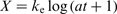
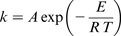
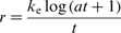
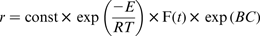
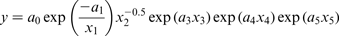
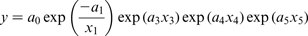
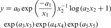
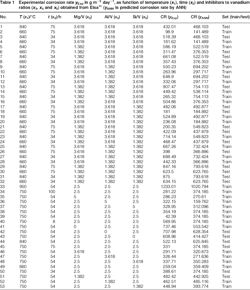
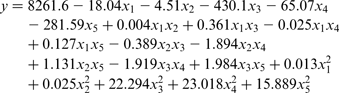
Corrosion rate as a function of different variables is given in Table 1. In the present work, three kinetic mathematical models are constructed. Parabolic kinetics, linear kinetics and logarithmic kinetics were used. These models are listed respectively as follows
1


Experimental corrosion rate y Exp in g m− 2 day− 1, as function of temperature (x 1), time (x 2) and inhibitors to vanadium ratios (x 3, x 4 and x 5) obtained from Eisa 11 (y ANN is predicted corrosion rate by ANN)
Artificial neural network methodology
The corrosion rate data were also used as feed for building the ANN. An ANN is an intelligent data driven modelling instrument that is able to arrest and represent complex and non-linear input/output relationships; they simulate the learning process of the human mind. Like the brain, the network structure composed of several processing features is called neurons or nodes. 14 The simplest custom of ANN is the linear model. A neural network with no hidden layers, and an output with dot product synaptic function and identity activation function, actually implements a linear model. The weights correspond to the matrix and the thresholds to the bias vector. When the network is performed, it effectively multiplies the input by the weights matrix then adds the bias vector. The linear network delivers a good benchmark against which to compare the performance of neural networks. The multilayer perceptrons (MLP) network trained using back propagation algorithm is a widely used network type and is commonly applied to all types of engineering as well as research modelling problems. A radial basis function neural network is a new class of robust neural network that has been used to a restricted extent in modelling various research problems. 15 The neural network model used in this study was created using STATISTICA 7 software package; it is a broad, state-of-the-art, influential and extremely fast neural network data analysis package. This feature has different options and subsoftware. One of them is an Intelligent Problem Solver (IPS). Unit activation levels are (by default) presented in colour: red for positive activation levels and green for negative. Triangles pointing to the right indicate input neurons. These neurons perform no processing and simply introduce the input values to the network. Squares indicate dot product synaptic function units (e.g. as found in MLP). Circles indicate radial synaptic function units. Small open circles that represent input and output variables are clarified using a small open circle joined to the corresponding input or output neuron. In some conditions, a number of neurons are joined to a single input or output variable. These networks were constructed using different activation functions such as sigmoid, hyperbolic, exponential, step, ramp, sine, square root, etc. Intelligent Problem Solver chooses the best activation function for network building. Each input comes via a connection that has a strength (or weight); these weights correspond to synaptic efficacy in a biological neuron. Each neuron also has a single threshold value. The weighted sum of the inputs is designed, and the threshold subtracted, to compose the activation of the neuron (also known as the post-synaptic potential of the neuron). The activation signal is passed through an activation function (also known as a transfer function) to produce the output of the neuron. If the step activation function is used (i.e. the neuron's output is 0 if the input is < 0, and 1 if the input is ≥ 0), then the neuron acts just like the biological neuron described earlier (subtracting the threshold from the weighted sum and comparing with zero is equivalent to comparing the weighted sum to the threshold). It is also noticeable that weights can be negative, which implies that the synapse has an inhibitory rather than the excitatory effect on the neuron: inhibitory neurons are found in the brain. However, there also can be hidden neurons that play an internal role in the network. The input, hidden and output neurons need to be connected together. The key issue here is feedback. 16 A simple network has a feed forward structure: signals flow from inputs, forward through any hidden units, eventually attainment of the output units. Such a structure has firm behaviour.
Results and discussion
Mathematical and statistical considerations
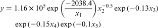
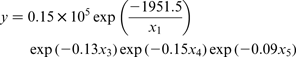
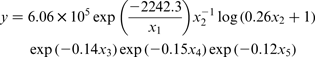
STATISTICA 7 software was used to estimate the coefficients of these models. This software was based on the Levenberg–Marquardt non-linear estimation least squares method. The maximum number of iterations was 1000, and the convergence criterion of 1 × 10− 6. The following equations are obtained
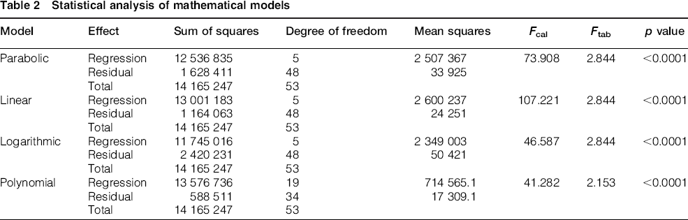
Statistical analysis of mathematical models
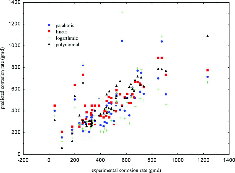
Experimental against predicted corrosion rate from mathematical regression
Artificial neural network considerations
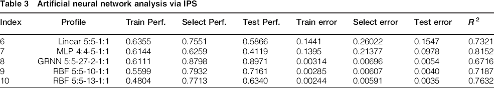
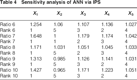
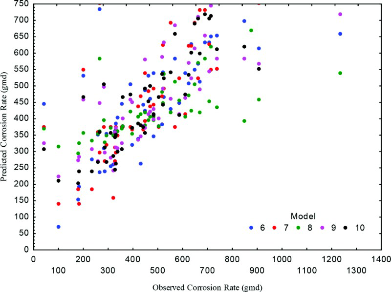
The ANNs were constructed using IPS. Many networks were tested and selected to represent the corrosion rate data. Figure 2 shows the created structure of ANN, while Tables 3 and 4 collected the most important data. Table 3 shows the investigation of each net ANN. The index represents a sole lifelong number assigned to each neural network when it is fashioned. The indices are assigned in chronological order. The profile is the most beneficial summary statistic, packing a great deal of information into a short piece of text. It tells us the network type, the number of input and output variables, the number of layers and the number of neurons in each layer. The arrangement is < type> < inputs>: < layer1>- < layer2>- < layer3>: < outputs>, where the number of layers may vary. For example, the profile MLP 4:4-5-1:1 signifies an MLP with four input variables and one output variable and three layers of 4, 5 and 1 units respectively. Columns Train Perf., Select Perf. and Test Perf. give the performance of the networks on the training, selection and test subsets respectively. It was shown that training sets did not give too much credence to the performance rate, which is often deceptively good (indicating overlearning). Furthermore, avoid using the test set performance to select models, as that overthrows the object of having it (which is to maintain some data not used for training or model selection, so that a composed final valuation of performance can be made). Use the performance measure on the selection subset to distinguish between, and choose between, networks. The meaning of the performance measure depends on the network type. It is the proportion of the prediction to observation standard deviations. Train error, Select error and Test error columns report the error rates on the subsets. The error rate is less directly interpretable than the performance measure, but is of more significance to the training algorithms themselves. Figure 3 shows the predicted corrosion rate against experimental one; the best results are obtained by MLP 4:4-5-1:1. (i.e. index 7). Table 4 shows the sensitivity analysis. It provides some information about the relative significance of the variables used in a neural network. In this analysis, the IPS test how the neural network would handle if each of its input variables was unavailable. The data set is submitted to the network recurrently, with each variable in turn treated as absent, and the subsequent network error is recorded. If a significant variable is canceled in this style, the error will increase an excessive deal; if an unimportant variable is removed, the error will not increase very much. As shown in Table 4, the sensitivity is stated in two rows: the Ratio and the Rank. The basic sensitivity number is the ratio. For each variable, the network is performed as if that variable is ‘unavailable’. Unavailability of a variable used by the model will apparently cause some decline in its performance. The ratio described is the ratio of the error with the variable absent to the ratio with its presence. Important variables have a high ratio, indicating that the network performance fails badly if they are not available. If the ratio is one or lower, then creating the variable ‘unavailable’ either has no effect on the performance of the network, or actually enhances it. The rank lists the variables in direction of importance (i.e. order of descending ratio) and is delivered for convenience in interpreting the sensitivities. In the current work data, it was found that most variables have a sensitive effect on corrosion rate. The same behaviour was observed with the mathematical polynomial model.
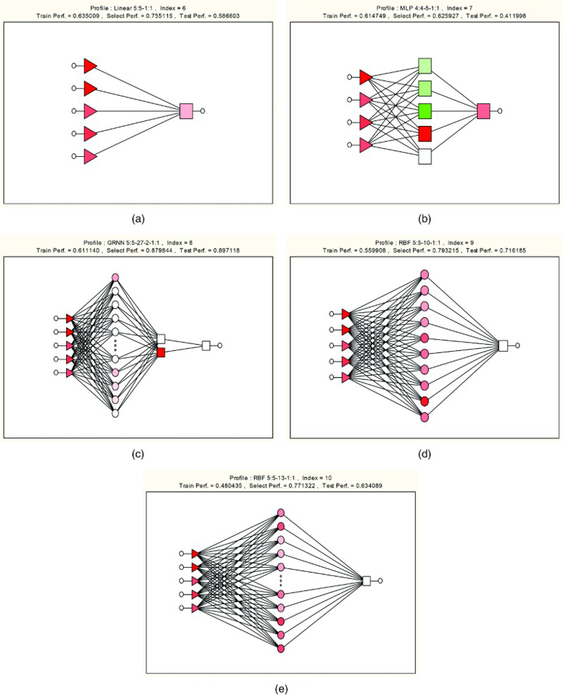
Artificial neural network created by Intelligent Problem Solver a Linear Model, b MLP Model, c GRNN Model, d RBF Model (5– 10 – 1), e RBF Model (5 – 13 – 1)
Artificial neural network analysis via IPS
Sensitivity analysis of ANN via IPS
Experimental corrosion rate against predicated by ANN
Optimum mathematical and ANN models
Mathematical and ANN analysis revealed that both methods represent the high temperature corrosion rate data in a powerful and effective manner. Figure 4 compares the mathematical polynomial models with the optimum ANN model. This indicates that both polynomial equations (from mathematical analysis) and MLP 4:4-5-1:1 (from ANN analysis) forecasted the corrosion rate values with higher correlation coefficients.
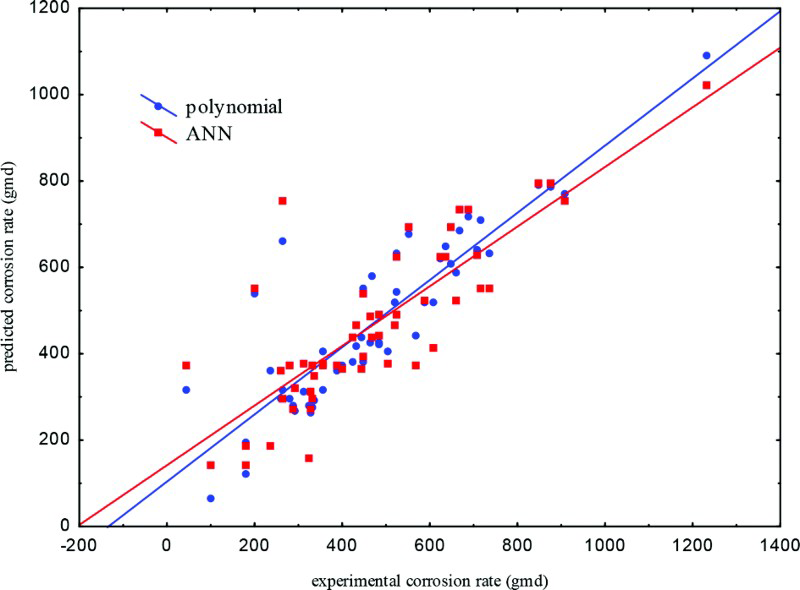
Experimental corrosion rate against predicated by optimum polynomial and optimum ANN models
Conclusions
The results obtained from weight loss measurements that were taken from the literature indicate that corrosion of steel in high temperature environment decreased with inhibitor concentration increase and increased with temperature and time of exposure. An attempt has been prepared to use mathematical regression, statistical analysis and ANNs to correlate the corrosion processes of steel as a function five operating conditions. For mathematical considerations, all suggested equations represented the corrosion rate data with different correlation coefficients. Polynomial model was the best one. In ANN studies, MLP 4:4-5-1:1 was the better architect.
Footnotes
Acknowledgement
This work was supported by Diyala University, Chemical Engineering Department, which is gratefully acknowledged.