Experience with the development and use of a simple DFN approach over a period of 30 years

Abstract

A contractual dispute on a tunnelling project more than 30 years ago was the impetus for the development of a program to generate discontinuity patterns. The purpose was to allow quantification of potential rockfalls, and determine appropriate rockbolt lengths and spacings. The simple discrete fracture network (DFN) program used measured or estimated statistical distributions of joint parameters to generate rock mass discontinuity patterns in any required two-dimensional section. The approach lends itself to a probabilistic analysis, and to use data determined quantitatively from the DFNs in the evaluation of risk. The development philosophy and application of the method will be described in the paper, supported by descriptions of several cases of practical engineering problems. Since a DFN does not represent the actual rock mass, but only one example of a ‘theoretical’ rock mass, multiple DFN representations need to be used to quantify engineering outputs.

Keywords

Discrete fracture network Instability prediction Tunnel Ventilation shaft Orepasses Tabular gold mine stopes Rock slopes Block caving cavability and fragmentation

This paper is part of a special issue on Discrete Fracture Network Engineering (DFNE)

Introduction

Discrete fracture networks (DFNs) have been in use in geotechnical engineering for many years. The DFN approach, which is described in this paper was developed in 1983 (Haines 1983; Grady 1983) to meet the need for quantification of potential rockfalls, and hence to determine appropriate rockbolt lengths and spacings, in a contractual dispute on a tunnelling project more than 30 years ago. Detailed discussions among a small group of SRK Consulting personnel resulted in a computer program, called JPLOT, for plotting possible joint traces in any two-dimensional section, making use of real data from field mapping of joints, and taking into account the statistical variability in these data. At that time, the capacity of computer hardware and quality of graphical output were rather limited – the program was written in Fortran and the output was to a drum plotter, but has now been rewritten to run in Mathcad. The DFN generating technique has been described in some detail by Haines (1984) and will not be repeated here. Input data for each joint set include dip direction, dip angle, dip and strike length, and spacing, as well as the ranges of each. Actual distributions of these data, if available from field mapping, can be used. Alternatively, ‘standard’ distributions of these parameters, based on field mapping all over the world, which have been published in the literature (for example Steffen, Kerrich and Jennings 1975; Call, Savely and Nicholas 1976; Priest and Hudson 1981; Hudson and Priest 1979; Hudson and Priest 1983), can be used. Typically accepted distributions are shown in Fig. 1. A common phrase used in geotechnical engineering associated with the use of very limited or poor quality site investigation data is ‘garbage in, garbage out’, implying that output in such cases is of no value. The application of DFNs is, however, one case in which this phrase is not considered to be appropriate. Since the “standard” distributions of joint structural parameters are known, a good estimate of the means and ranges of these parameters by an appropriately experienced geotechnical person will generally allow a good quality set of DFNs to be produced. Therefore, even with no measured data, it will often be possible to prepare satisfactory DFNs, which will be particularly useful at scoping and pre-feasibility levels.

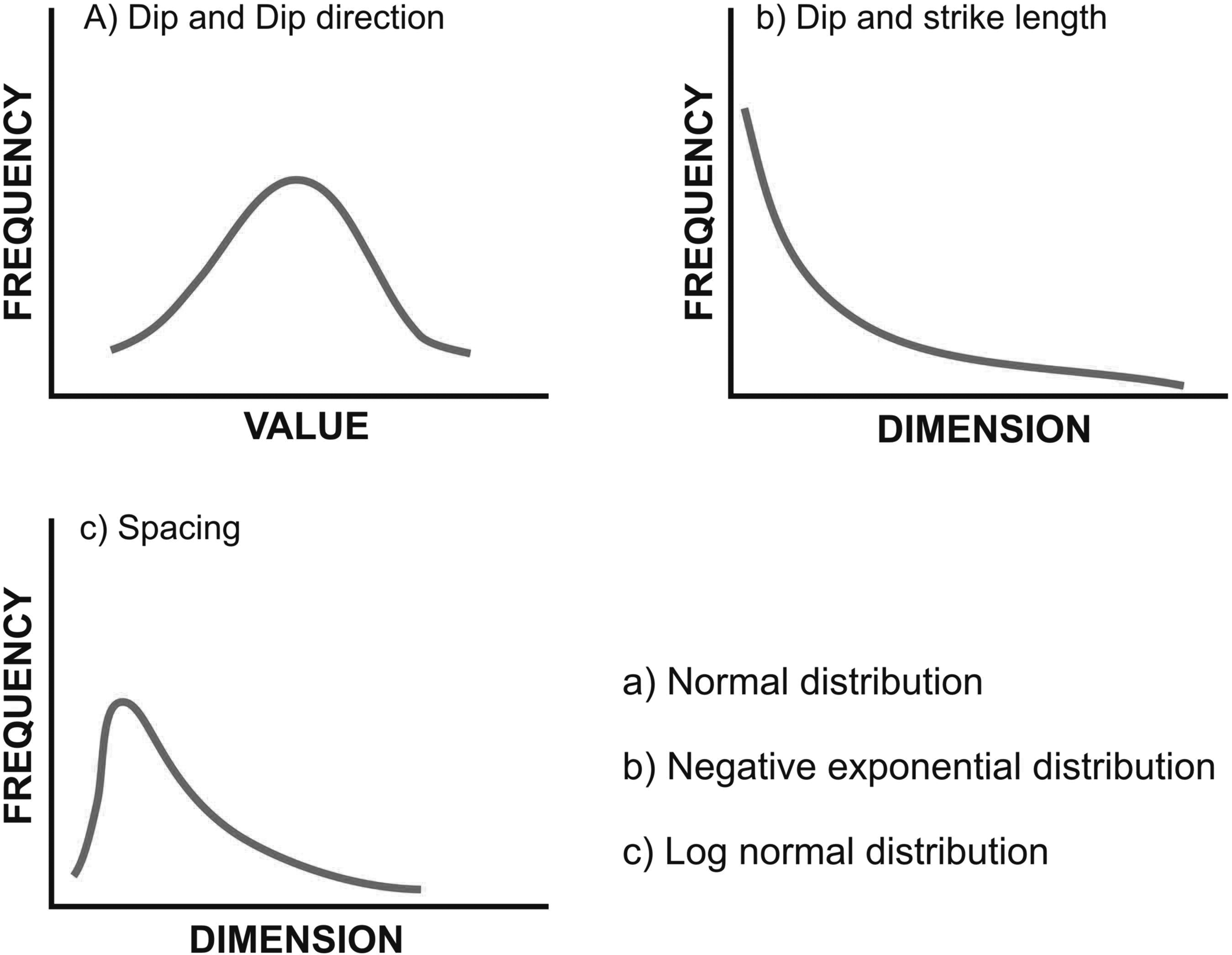
Typical distributions of jointing parameters in rock masses (Haines 1984)

Since the early development of the DFN method described by Haines (1984), substantial advances have taken place, and many valuable contributions have been made by sophisticated application of three-dimensional DFNs, and associated wedge and block limit equilibrium stability evaluations and numerical stress analyses (for example Dershowitz and Einstein 1988; Eberhardt, Stead and Coggan 2004; Pine, Coggan, Flynn and Elmo 2006; Grenon and Hadjigeorgiou 2000; Grenon and Hadjigeorgiou 2003; Vyazmensky, Elmo and Stead 2010). However, multiple applications of the simple method described in this paper have proved it to be very useful, and successful in all applications. This method may be considered to comply with the ‘simplicity’ rock mechanics design principle of Bieniawski (1992), suggesting that sophistication is not necessarily better.

Application of the simple DFN method

In the application of the method, joint traces are plotted to scale on appropriate two-dimensional sections through the excavation under evaluation. For example, for a tunnel, a horizontal axial section, a vertical axial section, and a vertical section normal to the tunnel axis would usually be satisfactory. The geometry of the excavation, to the same scale, is superimposed on the traces, and potentially unstable wedges and blocks identified, as illustrated in Fig. 2. This is a manual process, involving engineering judgement as to the potential instability of such blocks and wedges.

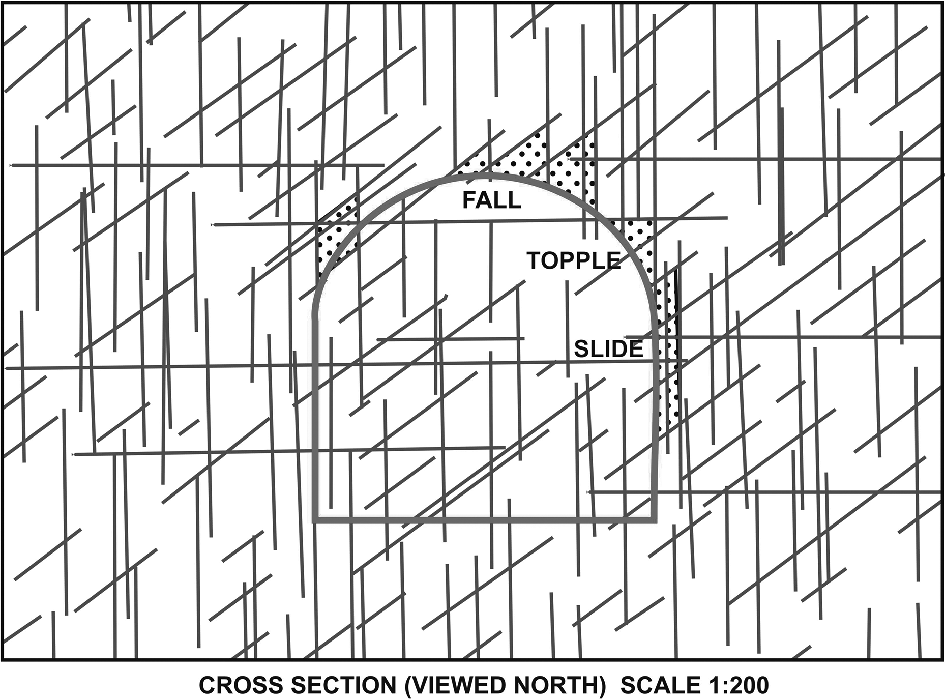
Identification of potentially unstable blocks and wedges on a discrete fracture networks (DFN) (Haines 1984)

Repeated superimpositions at different locations on the same trace plot, as illustrated in Fig. 3, can be used to identify alternative, or more, blocks and wedges.

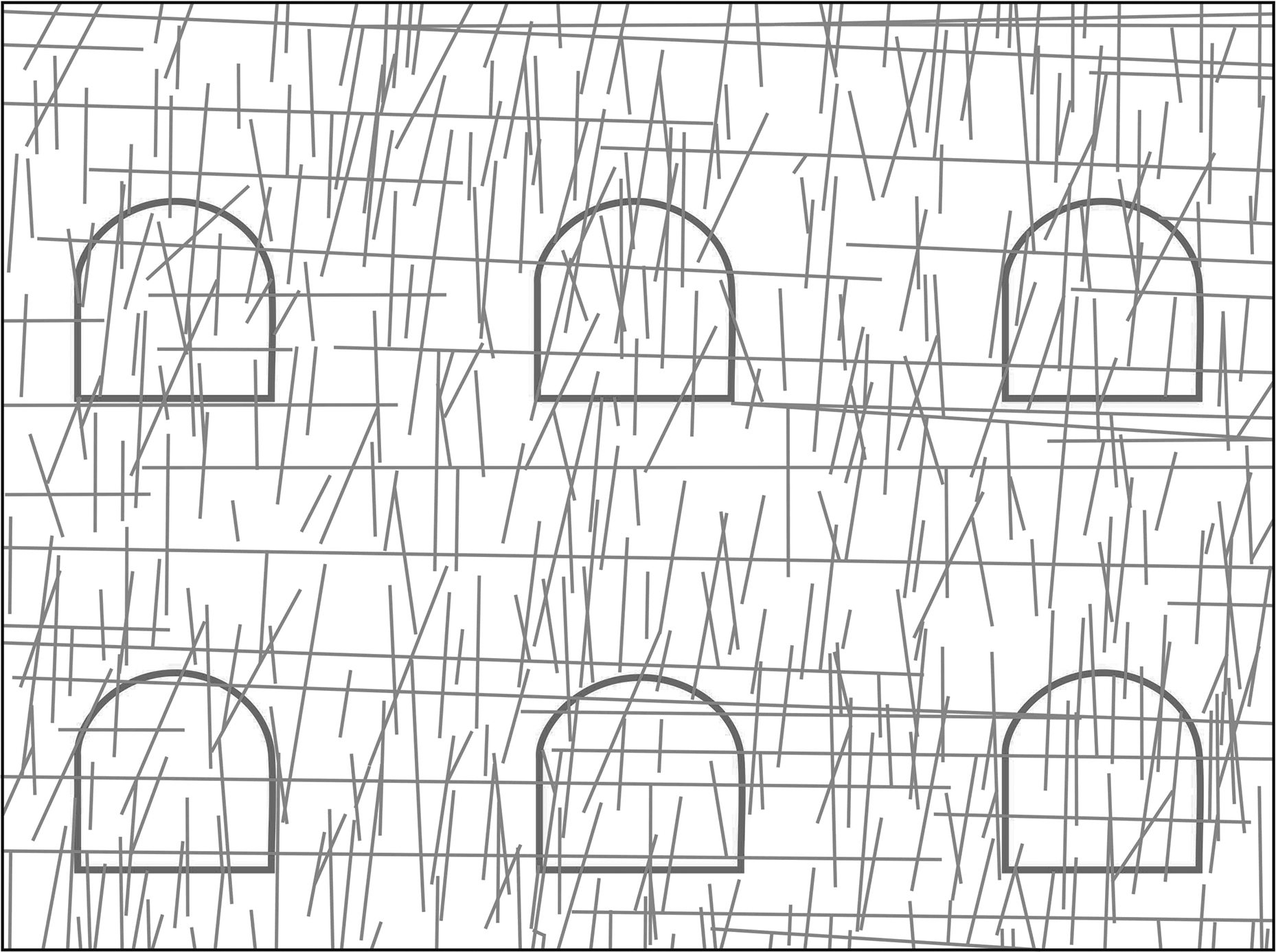
Excavation geometry at multiple locations on a discrete fracture networks (DFN) (Haines 1984)

Information of interest may be captured in this way: for example, the required information could be the depths of possible blocks behind the excavation surface; the face area of potentially unstable blocks. By producing joint trace patterns in orthogonal sections, it is possible to extend the simple two-dimensional method to three dimensions – information extracted could be the potential area of instability per metre length of tunnel, the potential volume of failure per metre length of tunnel, etc.

Results from the initial project were satisfactory, and the DFN plotting program has subsequently been used over a 30-year period on a variety of rock engineering projects, always with satisfaction.

Case studies of application of the JPLOT method

In the following sections, a variety of case studies will be presented. These case studies have been chosen to illustrate a wide range of application of the method.

Evaluation of potentially unstable blocks in a tunnel

Excavation of an inverted U-shaped railway tunnel was completed in the early 1980s. A number of rockfalls occurred during the tunnelling, and as a result it was necessary to evaluate the contractor's associated claims, and to determine the lengths and spacings of rockbolts required to ensure the permanent stability of the tunnel. Over its full length, the tunnel traversed five rock types with different geotechnical characteristics. The contractor's data on the rockfalls were not complete, and required evaluation. Based on this evaluation, it was concluded that the total volume of failure for 94% of the falls was 82 m³. The remaining 6% comprised specific falls owing to the influence of faults, and therefore could be ignored in the general analysis.

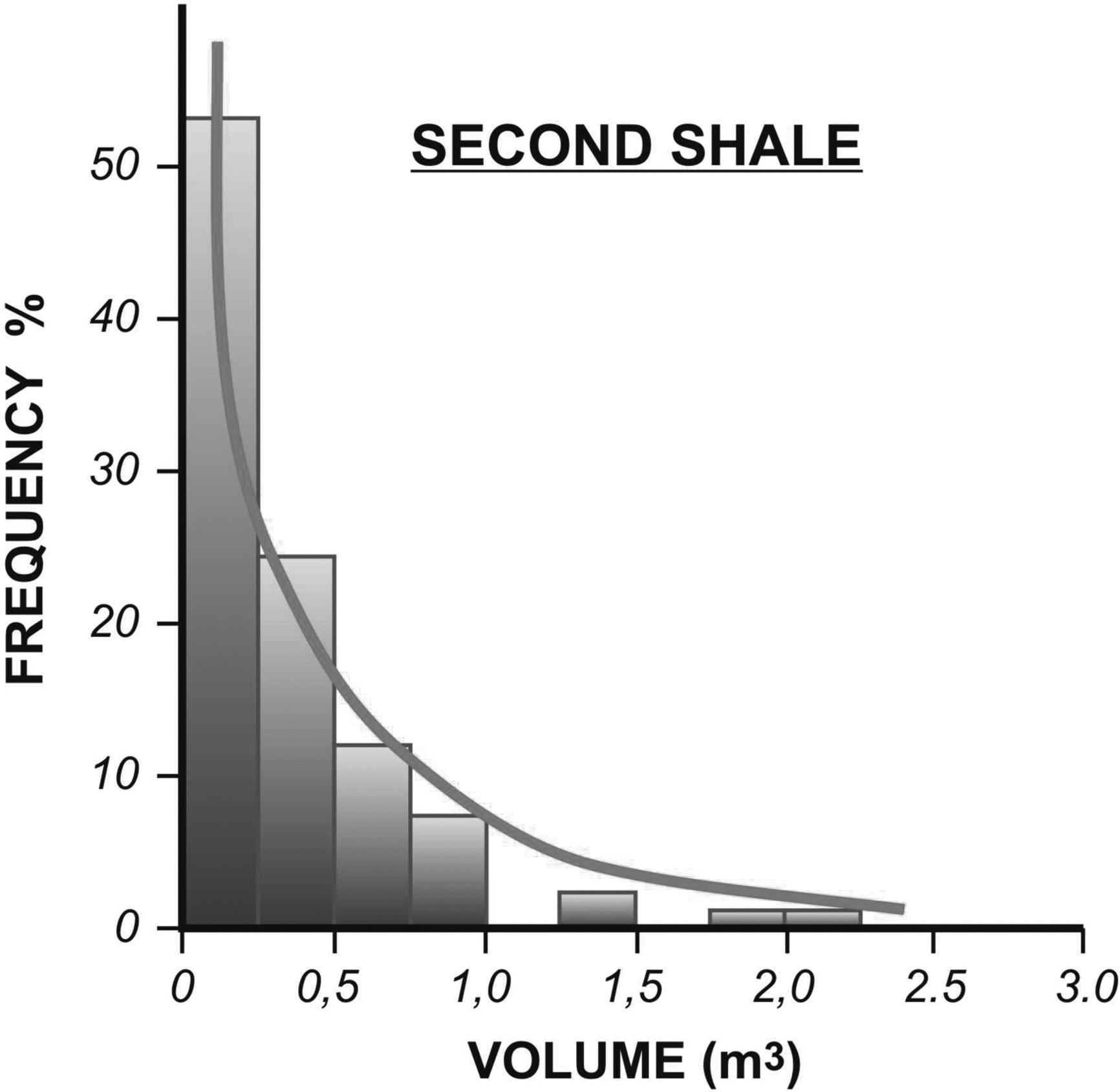
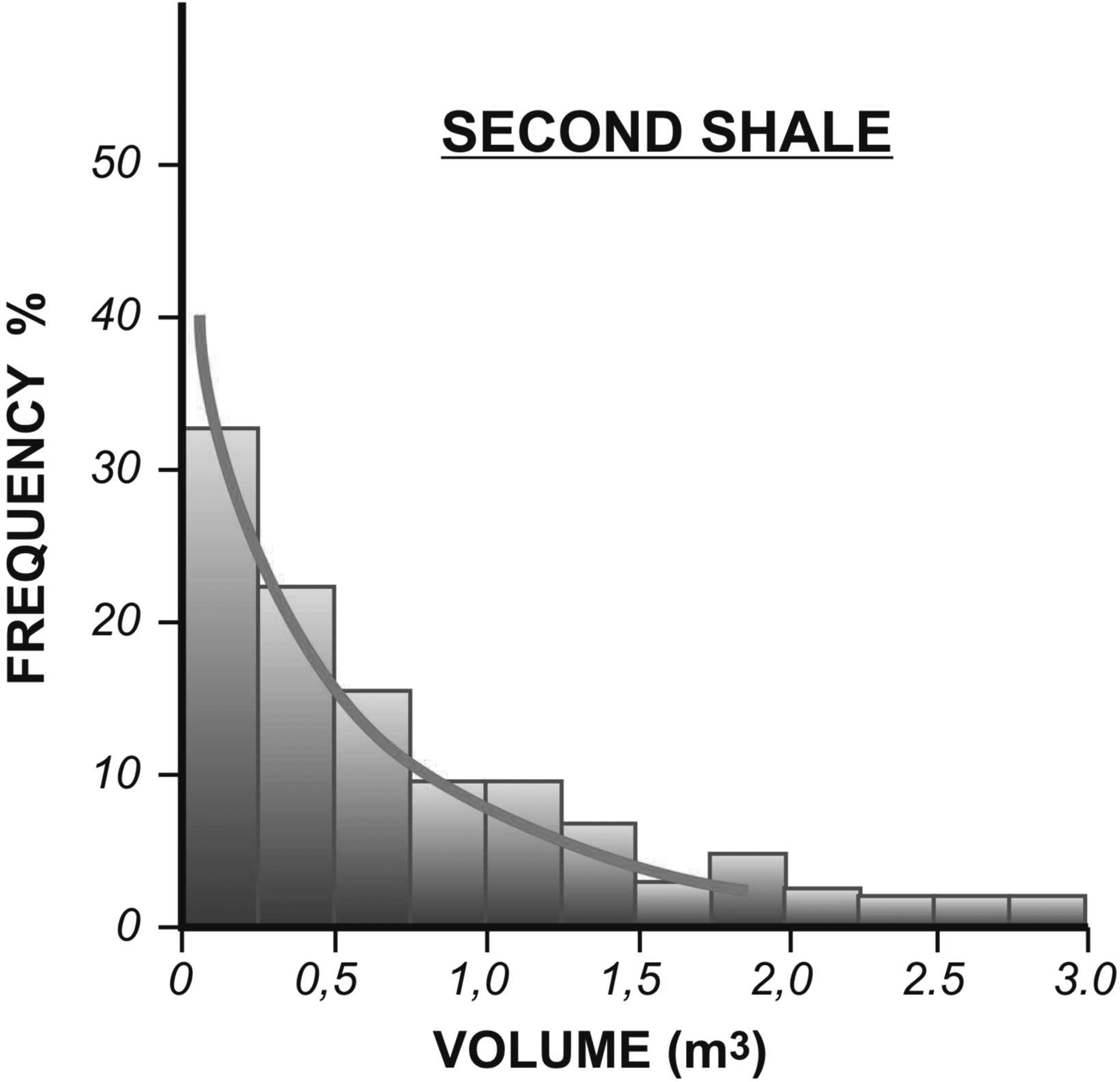
Based on the mapping of the tunnel face during excavation, jointing parameters were defined for the five rock types. These parameters were used in the generation of appropriate DFNs for the crown and sidewalls of the tunnel. Evaluation of potentially unstable blocks using these DFNs resulted in the determination of the predicted distributions of depths, areas and numbers of potentially unstable blocks in the tunnel crown and sidewalls. Examples of these for one of the rock types, the Second Shale, are shown in Fig. 4.

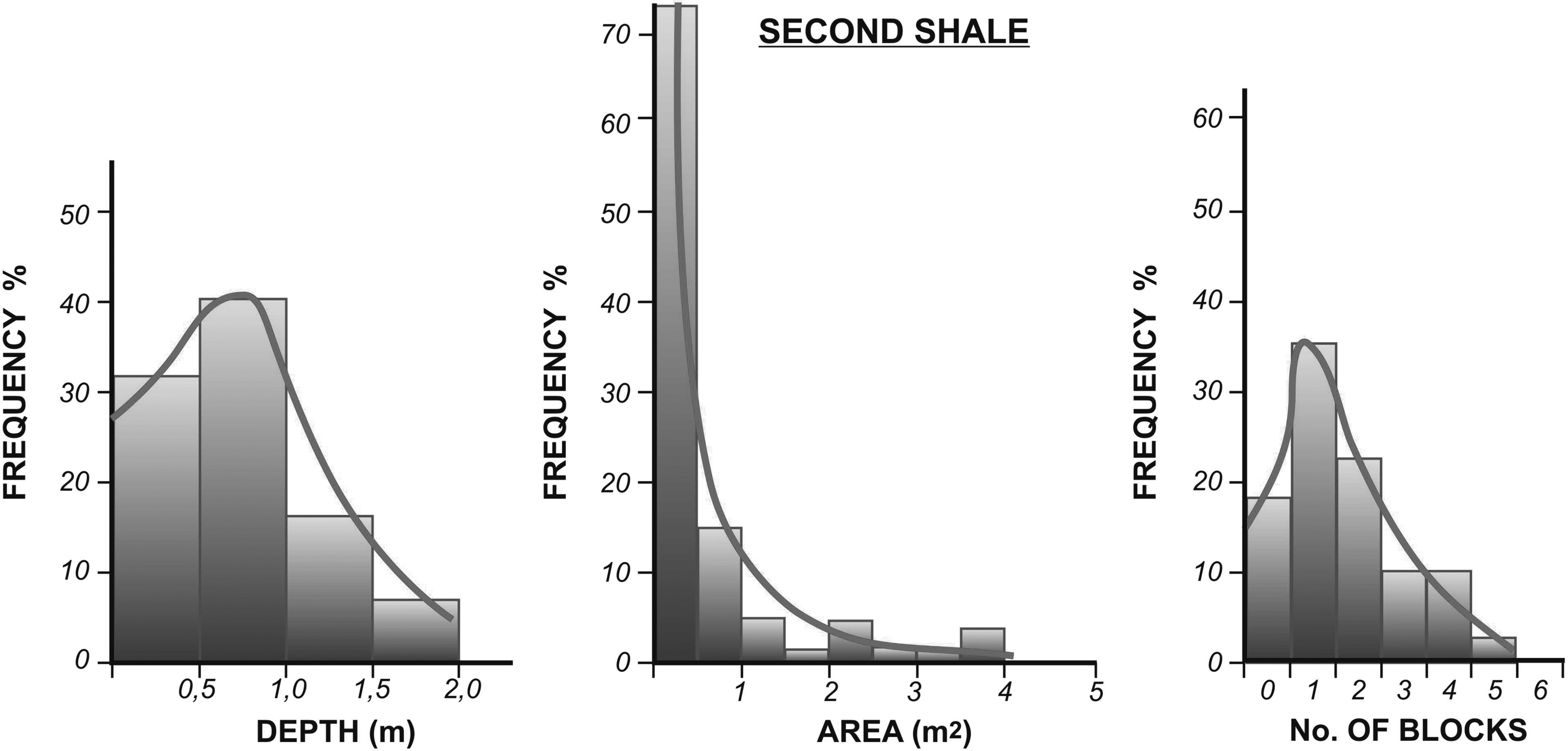
Distributions of block depth, face area and number of blocks per 3 m face advance, determined from discrete fracture networks (DFNs)

The prediction of volumes of potentially unstable blocks was a Monte–Carlo process, determined by randomly sampling the depth and area distributions, and using a volume factor between 1/3 and 1 to account for variations in block geometry. The volume of unstable material per 3 m face advance was determined by sampling the distributions of numbers of blocks per 3 m length and the volumes. These distributions are illustrated in Figs. 5 and 6.

Predicted distribution of volumes of individual potentially unstable blocks

Predicted distribution of total volumes of potentially unstable blocks per 3 m face advance

The total volume of potentially unstable material along the entire tunnel length could then be predicted by sampling the potentially unstable volume per 3 m of face advance ‘n’ times, where ‘n’ represented the number of 3 m advances in each rock type. The validity of the approach can be judged by the correlation between the predicted rockfall volumes and the actual volumes recorded during construction. At a 95% confidence level, the predicted total volume was 86 m³ compared with a volume of 82 m³ reported for 94% of the actual rockfalls that occurred.

Rockbolt lengths and spacings were determined, respectively, from the block depth distribution and block number distribution per 3 m face advance. The results corresponded well with assessments based on industry norms (for example Barton, Lien and Lunde 1974; Bieniawski 1984).

Prediction of potential breakout in a ventilation shaft

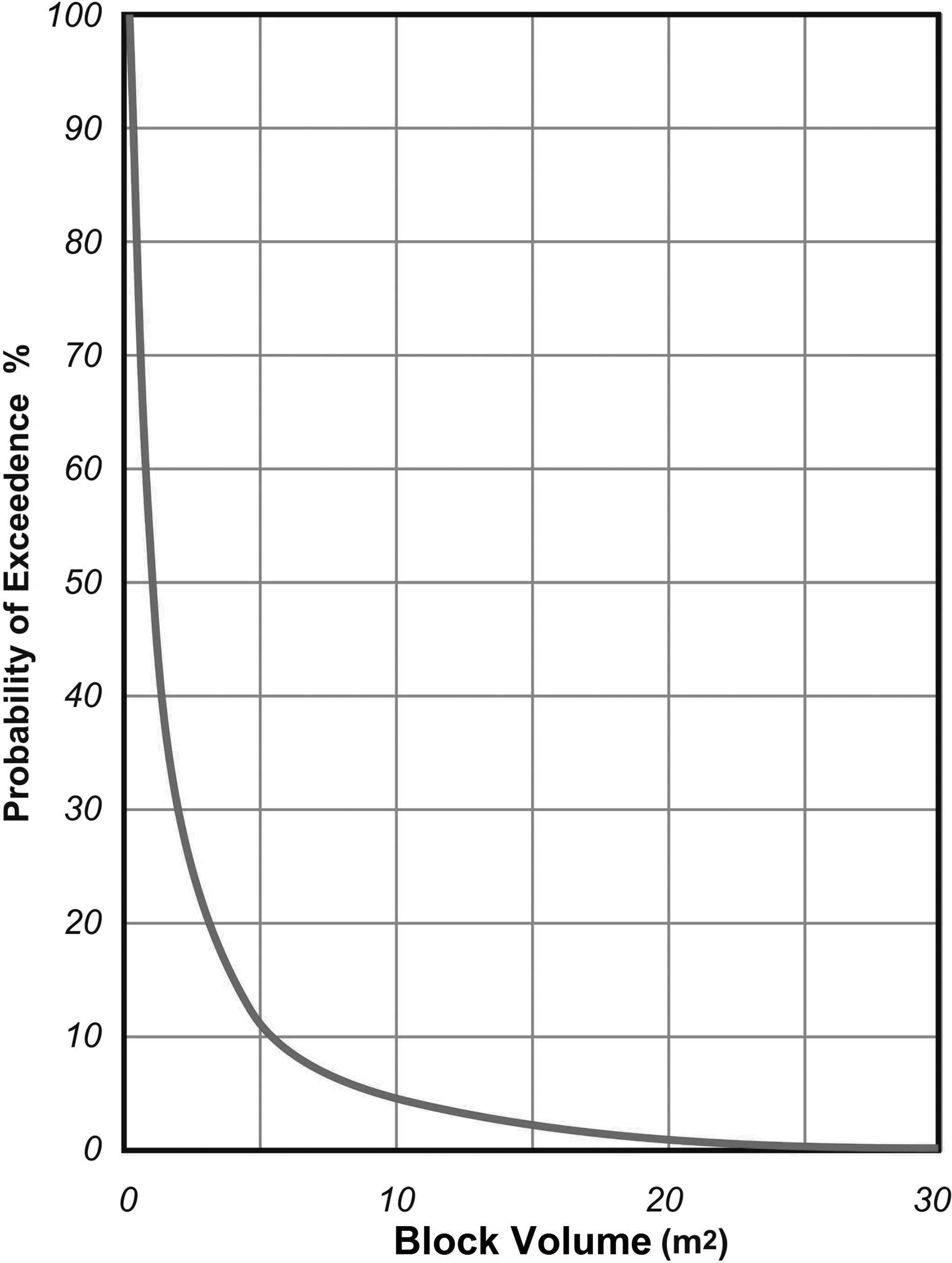
While minor rockfalls may not be a concern in a ventilation shaft since there is no access to such an excavation, a greater extent of instability may influence the effectiveness of the ventilation system. In such a case, a prediction of the likelihood of significant rockfalls is required, since it would determine whether the shaft should be lined or not. In this particular case study, input data for the evaluation were limited since no borehole had been drilled specifically to the shaft. General details of the geology, and of some of the jointing parameters, were, however, available for the rock mass. Making use of these data, and applying some experience-based judgement, DFNs were created and analysed in essentially the same way as described in Evaluation of potentially unstable blocks in a tunnel section above. From the DFN plots, potentially unstable blocks and wedges were identified and hence distributions of their sizes were obtained. Random sampling of these distributions allowed potential volumes of failure to be calculated, and hence the effect on the shaft cross-sectional area to be determined. From the investigation, the key outputs for decision making are the curves shown in Figs. 7, 8 and 9. Figure 7 shows a cumulative distribution graph from which the probability of the cross-sectional area of the shaft exceeding a certain value can be determined.

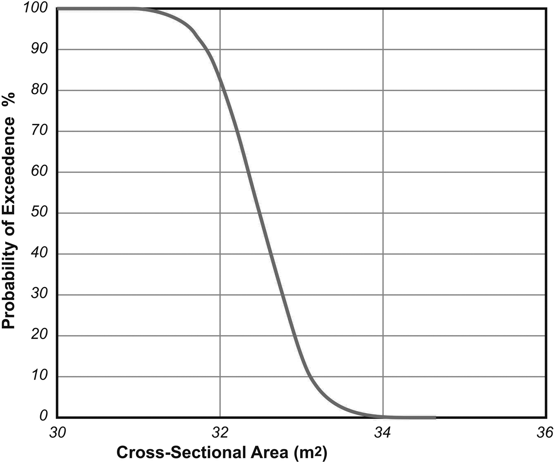
Probability of shaft cross-sectional area being exceeded

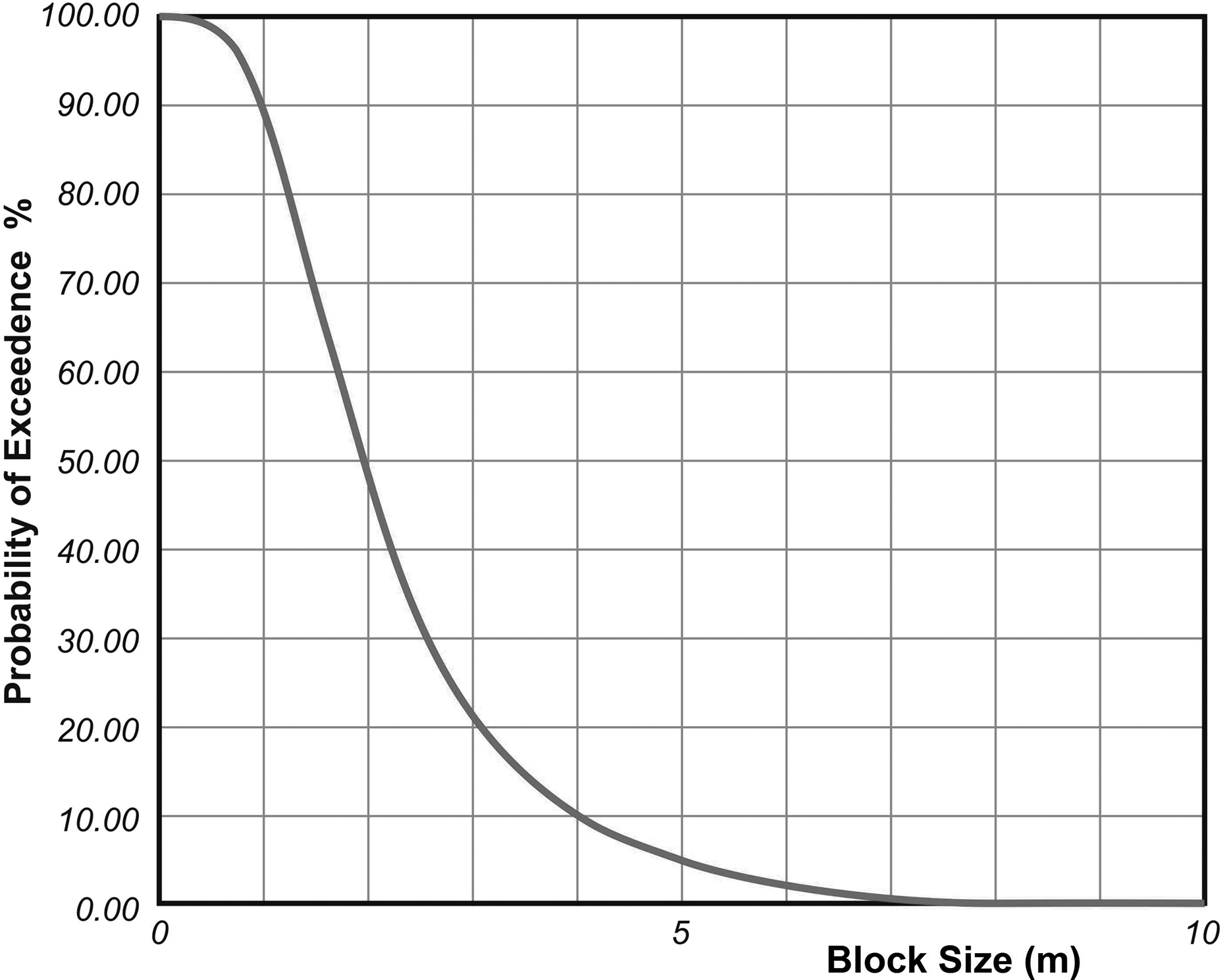
Probability of an unstable block exceeding a certain size

Probability of an unstable block exceeding a certain volume

The probability of occurrence of block sizes and volumes of failure, of significant importance in regard to the effective operation of the shaft, can be identified from Figs. 8 and 9.

This case is an example of a geotechnical problem in which, although sufficiently detailed and specific knowledge of rock mass parameters was inadequate for a conventional geotechnical evaluation, the DFN approach allowed a very realistic analysis to be carried out in a short time period.

The probabilities given in the three curves above are considered to have provided a satisfactory set of quantitative data on which the decision could be taken as to whether to line the shaft or not.

Prediction of cavability and fragmentation in a block cave mining project

The block or panel caving mining method has been increasing in popularity since it is the lowest cost massive mining method. In the assessment of the possibility of implementing this method, it is necessary to predict when the orebody will cave and what will be the block sizes and tonnages that will report at the drawpoints. Usually, this information is required at an early stage, often when very limited geotechnical information is available. This is a situation in which a DFN method may be considered to have great application.

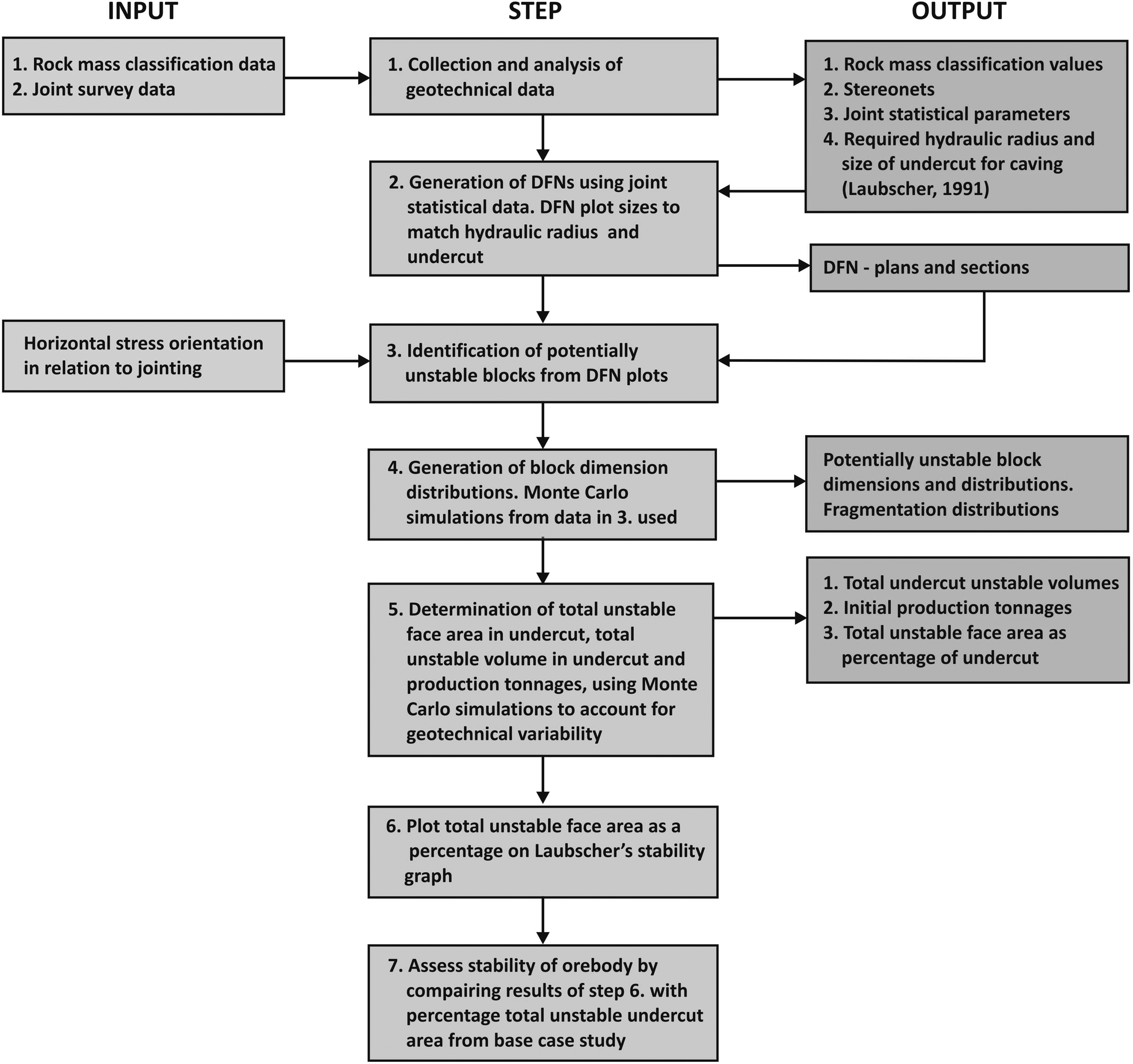
Butcher (2000) researched such a method, and tested the output against corresponding, known data. Much of his application involved the logic described in evaluation of potentially unstable blocks in a tunnel section, but he also included the effect of in situ stress, and correlation with rock mass classification outputs. The flow diagram summarising his method is shown in Fig. 10.

Flow diagram of the approach (modified after Butcher 2000)

Butcher (2000) applied the method to a ‘base case’ in which the actual performance was known. His DFN analysis predicted that the initial block cave tonnage should be 1191 t day^− 1. This compares reasonably well with the actual recorded value of 978 t day^− 1. Fragmentation distribution was not available for the base case mine, but was available from another kimberlite mine with similar orebody characteristics. The comparison between predicted and actual data in Fig. 11 shows the good quality of the prediction.

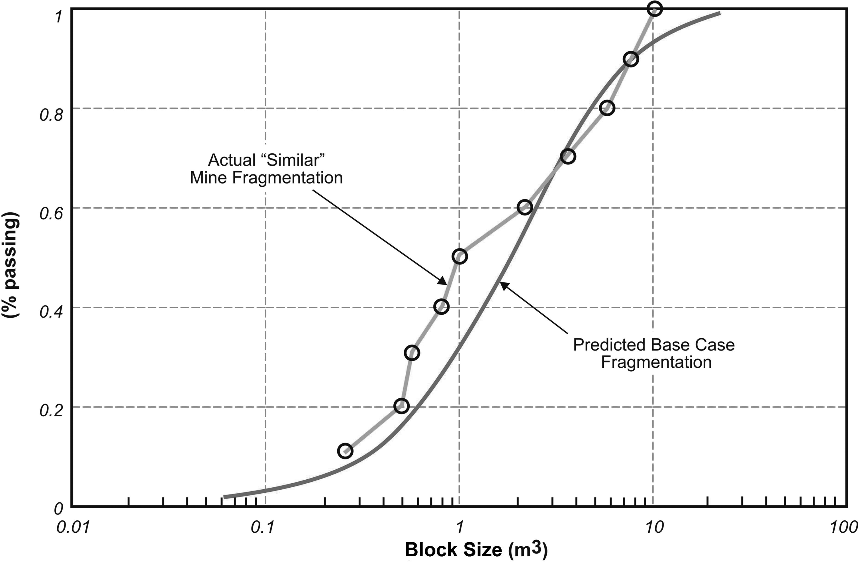
Comparison of predicted block size distribution with the distribution recorded at a similar kimberlite mine (modified after Butcher 2000)

Butcher states: ‘a major input into the tonnage calculation was the total face area of unstable blocks occurring in the back. This has been calculated at 15% of the undercut area, the undercut area being determined by the caving hydraulic radius (as given by Laubscher's stability diagram (Laubscher 1990). It can be concluded that 15% of the undercut back area must consist of unstable blocks to initiate caving. Further observation indicated that 80% of the back must be made up of unstable back blocks to continue the process of caving and cause propagation’.

In the mining industry, prediction of cavability, required hydraulic radius, fragmentation distribution and initial and production tonnages are still largely empirically based. This is not a criticism, but this case study demonstrates that application of a DFN approach could offer an additional or alternative approach that could add confidence in the prediction of the required performance data.

Prediction of the stability of orepasses under high stress conditions

Rock passes for ore and waste in mines are usually given very little attention with regard to strategy and design (Hadjigeorgiou and Stacey 2013). Designs are often simply lines on engineering drawings, without any geotechnical basis. Consequently, there is usually no geotechnical information associated with passes, and no documentation on the condition of the pass until a problem occurs.

As part of an investigation into issues associated with mining at great depths (down to 5000 m), predictions were required as to how rock passes would perform at such depths. At these depths, in situ stress magnitudes are high enough to cause failure of the intact rock, resulting in breakouts (locally referred to as ‘dog ears’) in the passes. The passage of rock material down the passes causes wear and additional scaling, and the passes may ‘grow’ to large span openings. In addition to the stress effects, the stability of the passes is significantly affected by the geological structure of the rock mass, and the orientation of the pass relative to this structure. To evaluate this latter aspect, a DFN approach was used. There was no specific information available for the rock mass structure, and generic or typical parameters were therefore used, and, of course, the ‘standard’ jointing parameter distribution shown in Fig. 1.

The extent of stress-induced breakouts at different mining depths was estimated, resulting in an estimated breakout span for each depth considered. These geometries represented the starting points for the DFN analyses. Application of the methods described in Evaluation of potentially unstable blocks in a tunnel section allowed the prediction of the following: •

the influence of pass diameter on stability and scaling

•

the influence of pass orientation, relative to strata dip, on stability and scaling

•

the influence of depth (stress) on stability and scaling.

From a research project into pass performance on mines, a database of pass behaviour was compiled (Joughin and Stacey 2004), which has provided a source of information for comparison with the results of the DFN analyses. The results of the comparison are shown in Fig. 12. The trends of the observed data and the predicted data are very similar, confirming the value of a DFN approach. It is to be noted that the quality of information available from mines was poor, which is a reason for the large scatter in the observational data points on the graph.

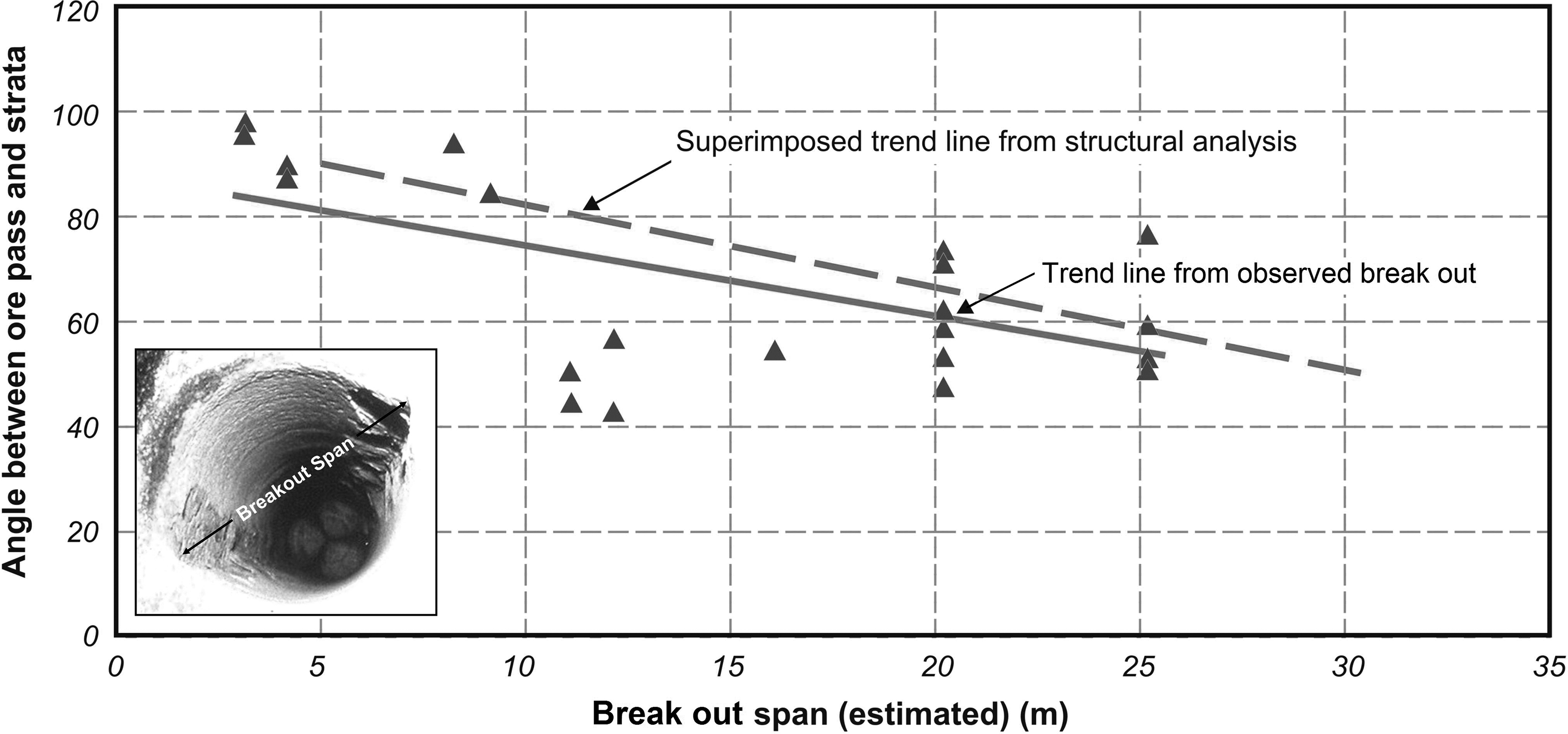
Comparison between data on observed scaling and data predicted from DFNs (Stacey, Wesseloo and Bell 2005)

This case demonstrates the power and usefulness of a DFN approach when poor or little specific geological structural data are available.

Prediction of rockfalls in deep level tabular gold mine stopes

Rock falls in tabular stopes in deep level gold mines usually result when unstable rock blocks are defined by the interaction between natural joints in the rock mass, and also interaction between these joints and stress-induced fractures. It is surprising that there were no documented, published data on jointing parameters before the work by Gumede (2006) and Gumede and Stacey (2006). Without such data, it is not possible to carry out a satisfactory engineering support design to contain such falls.

Gumede (2006) carried out conventional mapping of joints in a gold mine to establish the jointing statistical parameters. Using these statistics, he created DFNs and evaluated the potential for rock falls using the techniques described in evaluation of potentially unstable blocks in a tunnel section. These data were used to predict the heights of potential falls into the stope hangingwall. Mines are required to report this value in the event of a significant fall, and certainly when an accident occurs owing to a rock fall. These values provided the basis for comparison between the DFN predictions and measured heights. The empirical data presented by Daehnke, Van Zyl and Roberts (2001) indicated a height for rock falls of 1.2 m and for rockbursts of 1.8 m for stopes on one reef, and corresponding values of 1.0 and 2.2 m for stopes on another reef. The DFNs do not differentiate between static and dynamic conditions, and therefore the rockburst data of 1.8 and 2.2 m for the two stopes were applicable. The DFN method predicted heights of 1.8 and 2.2 m, agreeing exactly with the empirical data.

The analysis was taken further using a keyblock-based package (Esterhuizen and Streuders 1998) for the probabilistic assessment of gravity driven rock falls, and the evaluation of support effectiveness by Gumede and Stacey (2006). It was further extended to the prediction of the probability of occurrence of an accident (Stacey and Gumede 2006). Joughin, Jager, Nezomba and Rwodzi (2012a, 2012b) have further developed the approach for the probabilistic design of stope support in the Bushveld Complex platinum mines.

Prediction of break-back in rock slopes

All of the cases described above have dealt with underground excavations. The present, final case deals with rock slope stability. In near-surface excavations, stresses are low and therefore block confinement is limited. Failures of rock slopes in open pits are usually determined by geological planes of weakness, and in situ stresses are generally considered to be of minor importance. The problems of interest were the extent and volume of material involved in failure of three-dimensional jointed rock slopes (Armstrong and Stacey 2005). Data on break-back of slopes were available from small three-dimensional model rock slopes, which were tested under centrifuge loading (Stacey 1973, 1974). The DFN method was applied to these models using two sets of data: the first was the joint data assuming the typical joint statistical parameter distributions; the second was to use the actual joint geometries, since, in the model structure, there was no variation in jointing parameters. Rock slope failures in two models are shown in Fig. 13. Failure in a third model with a plane slope was controlled by the dip of the bedding planes.

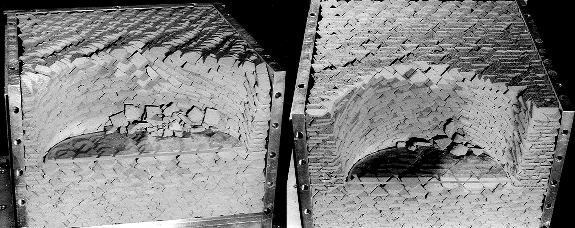
Slope failures in models with different plan radii of curvature (Stacey 1973)

The results from the DFN application to the model slopes are shown in Fig. 14 in the form of the break-back versus the plan radius of curvature of the slope, normalised to the height of the slope.

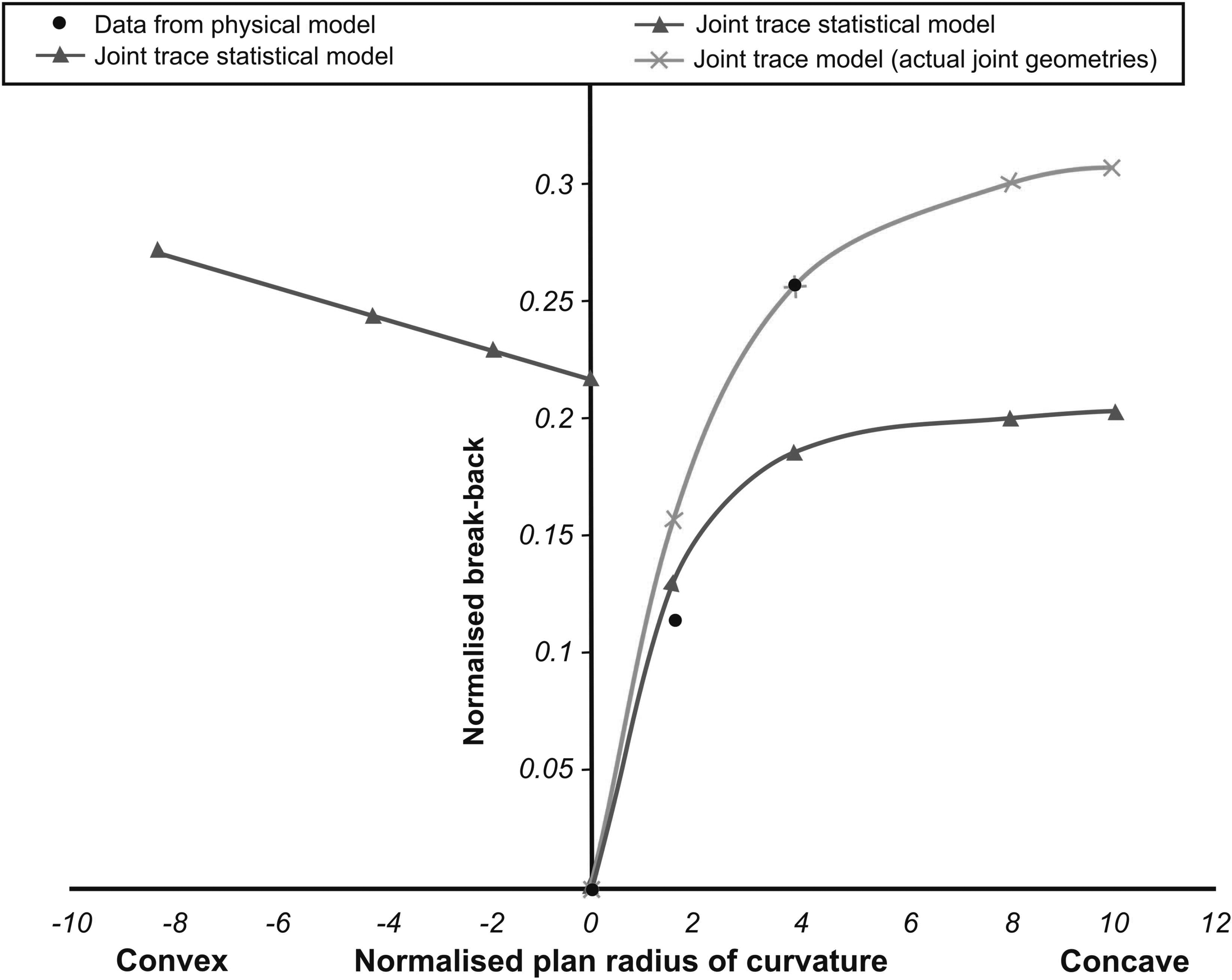
Predictions of break-back from DFN method, and measured break-backs in models (Armstrong and Stacey 2005)

There is close agreement between the physical model results and the predictions using the actual joint geometries. This gives confidence in the DFN method for prediction of the extent of slope failure. The outputs from DFN models, in which joint parameter distributions were used, expectedly result in smaller extents of failure, and may be considered to be more realistic for applications to real rock slopes. The completely different characteristics of concave and convex slopes are clear in Fig. 14, and the results indicate that failure is not inhibited when the concave plan radius of curvature exceeds 10 times the slope height.

The DFN method was applied to the real case of prediction of break-back in a vertical pit (Joubert, Freeman, Terbrugge and Venter 2008). The output from this analysis is shown in Fig. 15 in the form of the probability distribution of break-back. In a vertical pit operation, the stability of the walls is critical, and break-back must be designed against.

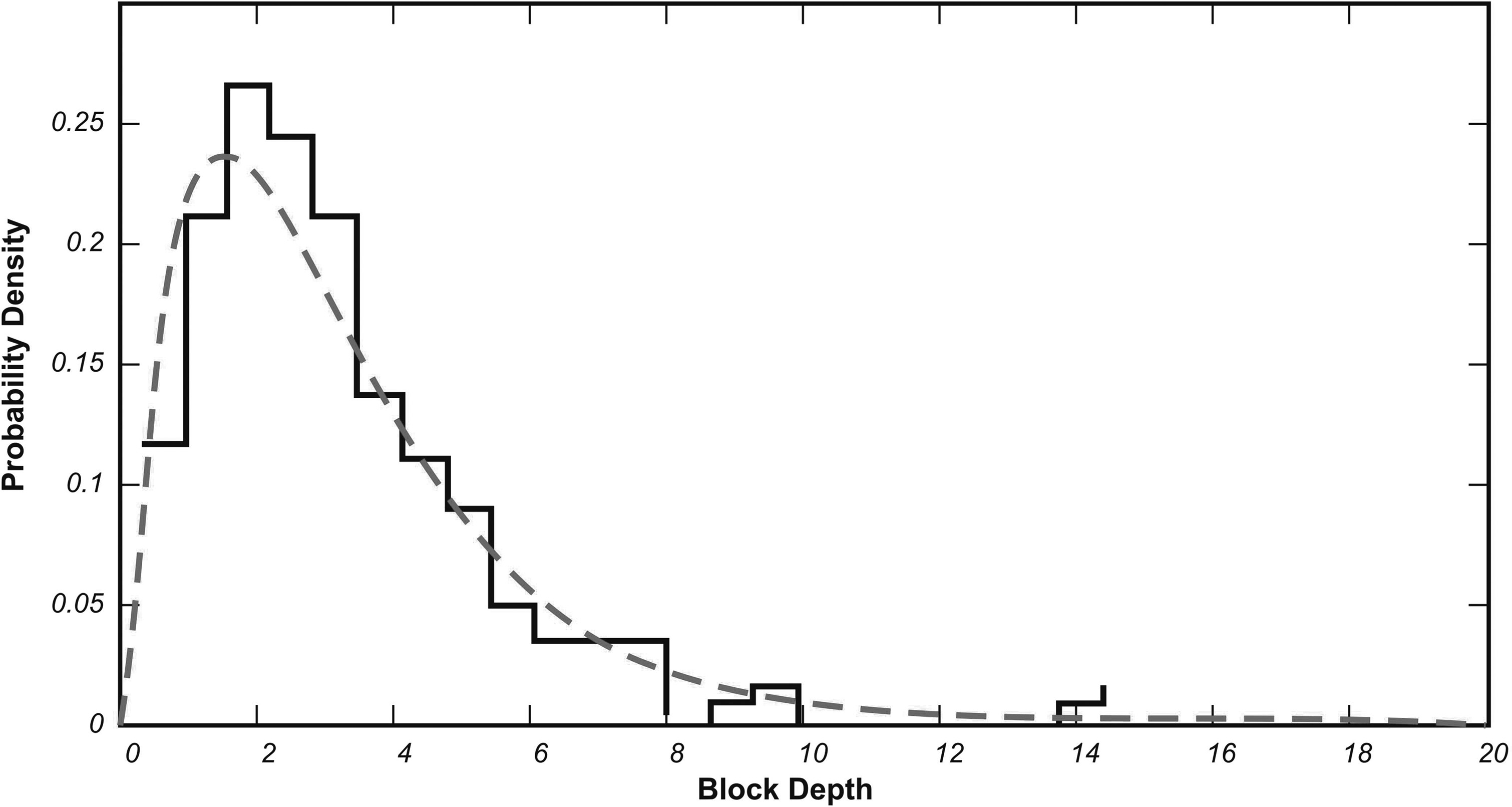
Probability distribution of predicted slope break-back (block depth) in a vertical pit from the DFN analysis (Joubert et al. 2008)

From Fig. 15, it can be seen that the DFN analysis predicts that there is a small probability of occurrence of a break-back of 14 m. When the pit reached a depth of 74 m below the pit collar, a significant sidewall failure occurred as shown in Fig. 16. The break-back, estimated to be about 14 m (validating the prediction from the DFN method), caused the premature termination of the vertical pit operation, and the requirement to convert to underground mining earlier than planned.

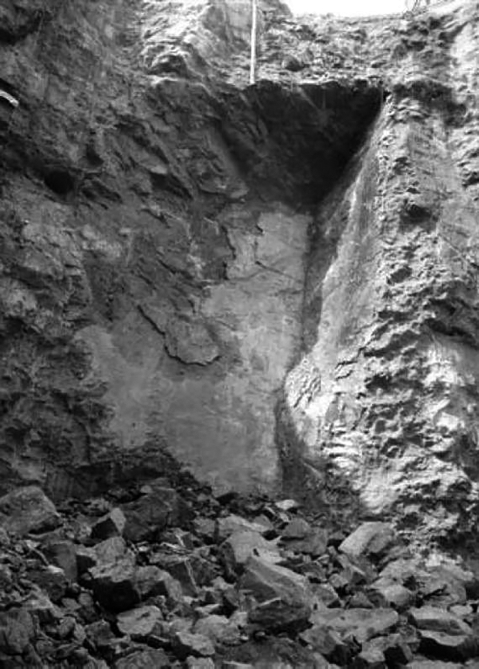
Large wedge failure from the sidewall of the vertical pit, visible face approximately 60 m in height

Discussion

The DFN technique described in this paper is a very simple one, particularly in comparison with the complex three-dimensional DFNs described in literature. However, the bulk of these complex DFNs have been used in conceptual research projects and not in applied engineering. It is simply not practical to numerically analyse a sufficient number of complex three-dimensional DFN's for design, owing to the extended computational times required for these models. Nevertheless, the case studies presented above have shown that the technique has produced predictions that have agreed remarkably well with actual observations and data. This simple method is considered to provide two major benefits:

The manual evaluation process, though perhaps tedious, allows the geologist and engineer to gain a good ‘feel’ for the quality of the rock mass and the extent of joint interaction. Often, this will indicate a better quality rock mass than would be interpreted from consideration of joint orientations only, and their potential geometric interaction. Geotechnical personnel will improve the quality of their engineering judgement in relation to the performance of the rock mass.

Being easy and quick to apply, the method lends itself to a probabilistic approach, and to use data determined quantitatively from the DFNs in the evaluation of risk. It must be clearly understood that, although a DFN, or theoretical rock mass, represents the rock mass based on the statistical data, obtained from measurements of structures within the rock mass, it is not the actual rock mass. It is only one of many potential rock masses based on those statistical data. The theoretical rock masses represented in the DFN plots in different cross-sections have no physical relationship with one another. Therefore in engineering design applications, to use only one, or few DFNs, even if they are sophisticated three-dimensional DFNs, is not correct, and may give significantly erroneous, invalid and unrepresentative results. It is necessary to make use of many DFNs, or at least a sufficient number, to be able to take into account the range of potential theoretical rock masses derived from the available statistical data. Application of numerous DFNs will allow probability distributions of design parameters to be determined, for example, distributions of depths, face areas, and volumes of potentially unstable blocks, as has been described in the case studies above. The method considers probability of occurrence rather than probability of failure, and this is considered to be a practical and conservative evaluation of potential failure.

Acknowledgements

The authors acknowledge the inputs of many geotechnical staff in the case studies described in this paper: G. Bell, R. Butcher, I. Cameron-Clarke, H. Gumede, A. Haines, G. Keyter, H. Kirsten, and J.Wesseloo.

This paper was originally presented at the first International Conference on Discrete Fracture Engineering (DFNE 2014) (19–22 October 2014, Vancouver, BC, Canada) and has subsequently been revised and extended before consideration by Mining Technology.

References

Armstrong

and Stacey

T. R.

2005. The extent and volume of three dimensional failures in rock slopes in which several sets of joints define the geological structure. In: Proc. 3rd Southern African Rock Engineering Symp., ‘Best practices in rock engineering’, Randburg, 201–209. [South African Institute of Mining and Metallurgy, Symposium Series S41].

Barton

, Lien

and Lunde

1974. Engineering classification of rock masses for the design of tunnel support, Rock Mechanics, 6, (4), 189–236.

Bieniawski

Z. T.

1984. Rock mechanics design in mining and tunnelling, London, A A Balkema.

Bieniawski

Z. T.

1992. Invited paper: principles of engineering design for rock mechanics. In: Rock Mechanics, Proc. 33rd U.S. Symp. on Rock Mech., (eds. Tillerson and Wawersik Virginia, Balkema, American Rock Mechanics Association, 1031–1040.

Butcher

R. J.

2000. A modelling method for predicting block cave cavability, initial fragmentation and production tonnage at a scoping study level. MSc Research Report, University of the Witwatersrand.

Call

R. D.

, Savely

J. P.

and Nicholas

D. E.

1976. Estimation of joint set characteristics from surface mapping data. In: Proc. 17th U.S. Symp. on Rock Mech., University of Utah: Utah, 2B2.1–2B2.9.

Daehnke

, Van Zyl

and Roberts

M. K. C.

2001. Review and application of stope support criteria, The Journal of the South African Institute of Mining and Metallurgy, 101, (5), 135–164.

Dershowitz

W. S.

and Einstein

H. H.

1988. Characterizing rock joint geometry with joint system models, Rock Mechanics and Rock Engineering, 21, 21–51.

Eberhardt

, Stead

and Coggan

J. S.

2004. Numerical analysis of initiation and progressive failure in natural rock slopes – the 1991 Randa rockslide, International Journal of Rock Mechanics and Mining Science, 41, 69–87.

10.

Esterhuizen

G. S.

and Streuders

S. B.

1988. Rockfall hazard evaluation using probabilistic keyblock analysis, The Journal of the South African Institute of Mining and Metallurgy, 98, (2), 59–63.

11.

Grady

L. A.

1983. The application of geostatistical techniques in the analysis of joint data. MSc Dissertation, University of the Witwatersrand.

12.

Grenon

and Hadjigeorgiou

2000. Stope design based on realistic joint networks. In: Proc. of MassMin 2000, Brisbane, AusIMM, 765–771.

13.

Grenon

and Hadjigeorgiou

2003. Open stope stability using 3D joint networks, Rock Mechanics and Rock Engineering, 36, (3), 183–208.

14.

Gumede

2006. Development of data sets on joint characteristics and consideration of associated instability for a typical South African gold mine. MSc Dissertation, University of the Witwatersrand.

15.

Gumede

and Stacey

T. R.

2006. Measurement of typical joint characteristics in South African gold mines and the use of these characteristics in the prediction of rock falls, The Journal of the South African Institute of Mining and Metallurgy, 107, (5), 335–344.

16.

Hadjigeorgiou

and Stacey

T. R.

2013. The absence of strategy in ore pass planning, design and management, The Journal of the South African Institute of Mining and Metallurgy, 113, 795–801.

17.

Haines

1983. The quantitative assessment of potential tunnel instability by extrapolation of rock mass discontinuity mapping. In Proc. Symp. on Rock Mech. in the Design of Tunnels, South African National Group of International Society & Rock Mechanics, 1–5.

18.

Haines

1984. The application of generated rock mass discontinuity patterns. In: Proc. 8th Regional Conf. for Africa on Soil Mechanics and Foundation Engineering,Harare, A A Balkema: Rotterdam, 13–21.

19.

Hudson

J. A.

and Priest

S. D.

1979. Discontinuities and rock mass geometry, International Journal of Rock Mechanics and Mining Science & Geomechanics Abstracts, 16, 339–362.

20.

Hudson

J. A.

and Priest

S. D.

1983. Discontinuity frequency in rock masses, International Journal of Rock Mechanics and Mining Science & Geomechanics Abstracts, 20, (2), 73–89.

21.

Joubert

J. S. C.

, Freeman

L. A.

, Terbrugge

P. J.

and Venter

2008. The Koidu Vertical Pit – Sierra Leone, in Proceedings of the Symposium on Surface Mining, Johannesburg Vol. 22, The Southern African Institute of Mining and Metallurgy.

22.

Joughin

and Stacey

T. R.

2004. The behaviour of ore passes in deep level tabular mines. In: Proceedings of the Second International Seminar on Deep and High Stress Mining, Johannesburg, South Africa, The Southern African Institute of Mining and Metallurgy, 395–411.

23.

Joughin

, Jager

, Nezomba

and Rwodzi

2012b. A risk evaluation model for support design in Bushveld Complex underground mines: part II – model validation and case studies, The Journal of the South African Institute of Mining and Metallurgy, 112, (2), 95–104.

24.

Joughin

, Jager

, Nezomba

and Rwodzi

2012a. A risk evaluation model for support design in Bushveld Complex underground mines: part I – description of the model, The Journal of the South African Institute of Mining and Metallurgy, 112, (2), 83–94.

25.

Laubscher

D. H.

1990. A geomechanics classification system for the rating of rock mass in mine design, The Journal of the South African Institute of Mining and Metallurgy, 90, (10), 257–273.

26.

Pine

R. J.

, Coggan

J. S.

, Flynn

Z. N.

and Elmo

2006. The development of a new numerical modelling approach for naturally fractured rock masses, Rock Mechanics and Rock Engineering, 39, (5), 395–419.

27.

Priest

S. D.

and Hudson

J. A.

1981. Estimation of discontinuity spacing and trace length using scanline surveys, International Journal of Rock Mechanics and Mining Science & Geomechanics Abstracts, 18, 183–197.

28.

Stacey

T. R.

1973. Stability of rock slopes in mining and civil engineering situations. DSc (Eng) Thesis, University of Pretoria..

29.

Stacey

T. R.

1974. The behaviour of two- and three-dimensional model rock slopes, Quarterly Journal of Engineering Geology, 8, 67–72.

30.

Stacey

T. R.

and Gumede

2006. Evaluation of risk of rock fall accidents in gold mine stopes based on measured joint data, The Journal of the South African Institute of Mining and Metallurgy, 107, (5), 345–350.

31.

Stacey

T. R.

, Wesseloo

and Bell

2005. Predicting the stability of rockpasses from the geological structure, The Journal of the South African Institute of Mining and Metallurgy, 105, (11), 803–808.

32.

Steffen

O. K. H.

, Kerrich

J. E.

and Jennings

J. E.

1975. Recent developments in the interpretation of data from joint surveys in rock masses. In: Proc. 6th Regional Conf. for Africa on Soil Mechanics and Foundation Engineering, South African Institution of Civil Engineers, Balkema, Rotterdam, 17–25.

33.

Vyazmensky

, Elmo

and Stead

2010. Role of rock mass fabric and faulting in the development of block caving induced surface subsidence, Rock Mech. Rock Eng., 43, 522–556.