
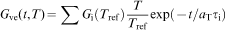
Abstract
A simple viscoplastic model for the stress–strain behaviour of filled rubber is presented. It consists, for a given strain, of additive contributions to stress from hyperviscoelasticity and time independent hysteresis. Rubber components are often subjected to scragging, i.e. preconditioning to a large strain, before carefully assessing their load deflection behaviour and comparing it to specification. The choice of scragging strain, however, affects the load deflection behaviour. It is found that this effect may be approximately captured, for modelling purposes, by regarding the modulus of the time-independent hysteresis contribution to be a function of the scragging strain and the time elapsed since scragging.
List of symbols
shift factor, a function of temperature, given by the Williams–Landel–Ferry equation (dimensionless)
elastoplastic secant shear modulus at ∼100% shear strain, MPa
elastoplastic parameter controlling the rate of decrease in modulus as the strain is increased (dimensionless)
elastoplastic parameter controlling the strain below, which the modulus asymptotes to a plateau (dimensionless)
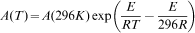
activation energy for elastoplastic contribution, J mol−1
shear modulus, MPa
storage (ratio of in phase stress amplitude to strain amplitude)
loss (ratio of out of phase stress amplitude to strain amplitude)
coefficient in Prony series expression for relaxation modulus
time independent part of relaxation modulus Ghve(t)
viscoelastic parameter equal to the gradient of relaxation modulus versus natural logarithm of time, MPa
viscoelastic parameter controlling power law contribution to relaxation modulus, MPa
first strain invariant equal to
 (dimensionless)
discretisation parameter equal to the ratio of consecutive relaxation times τi/τi−1 in the Prony series (dimensionless)
viscoelastic parameter being the exponent in the power law contribution to the relaxation modulus (dimensionless)
gas constant, 8·314 J K−1 mol−1
time scale used in Boltzmann's integral, s
time, s
absolute temperature, K
strain energy density, J m−3
loss angle equal to tan−1 (G″/G′) (dimensionless)
volume fraction of filler (dimensionless)
shear strain

amplitude (dimensionless)
extension ratio (dimensionless)
extension ratio in the ith principal direction
shear stress

amplitude, MPa
relaxation time, s
minimum and maximum considered times for applicability of the viscoelastic model
Subscripts
hyperelastic
viscoelastic
combined hyperelastic and viscoelastic
elastoplastic
Introduction
The general aim is a simple time domain viscoplastic model capable of capturing those aspects of the stress–strain behaviour of filled rubber of greatest relevance to engineering applications for implementation in three-dimensional non-linear finite element analysis using standard material models.
It is customary to subject many rubber engineering components to one or more cycles of deformation, somewhat greater than those anticipated in service, before releasing them for use. This may be intended as a test of integrity. It can also serve the purpose of achieving a representative level of stress softening and set, following which the load deformation behaviour is expected to be reasonably stable and representative of service conditions. This procedure is known as ‘scragging’, a term that rubber technologists seem to have borrowed from the metal spring industry (see for example Refs. 1 and 2), for which it refers to a prestress to cause yielding of the surface layers of the material, resulting in a permanent ‘set’, improved fatigue life and reduced risk of sagging. For both metal springs and rubber components, the load deflection behaviour is usually only carefully assessed and compared to specification after scragging. ISO 4664 (Ref. 3) states that rubber testpieces ‘should be mechanically conditioned (sometimes referred to as “scragging”) before testing, to remove irreversible “structure”. The conditioning should consist of at least six cycles at the maximum strain and temperature to be used in the series of tests’. The effect of scragging on stiffness and damping, and the subsequent recovery in these properties over time, has received much attention in the literature on the use of filled rubber in high damping elastomeric bearings for isolating structures from earthquakes. Unfortunately, this literature provides mainly general information, since the materials are varied and normally proprietary, and the tests tend to be neither carried out nor interpreted by rubber specialists. The AASHTO Guide Specifications for Seismic Isolation Design (1999)4 define the ‘scragging modification factor’ as the value of the property of the unscragged bearing divided by that of the scragged bearing and assume that the effect of scragging depends on the material and the recovery time. Constantinou et al.5 published a study on the concept of property modification factors that included the effect of scragging and formed the basis of the concept and values given in the AASHTO Guide.4
In this work, values for the parameters are fitted to dynamic shear stress–strain data for a filled natural rubber (NR) vulcanisate, designated EDS16 (TARRC Datasheets);6 the formulation is given in Table 1. Scragging the rubber is known to reduce its subsequent stiffness, an effect which has been comprehensively studied by Kingston.7 The purpose of this paper is to investigate whether his data on the effects of different scragging strains can be accommodated within the model proposed by Ahmadi et al.8, 9 (Fig. 1) by generalising the existing set of parameters to become functions of the scragging strain.
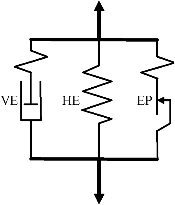
Representation of model as viscoelastic (VE), hyperelastic (HE) and elastoplastic (EP) contributions connected in parallel
Composition of rubber
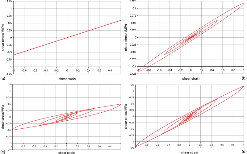
Since the mode of deformation in this paper was fully symmetrical cycling at about zero shear strain, there is no issue of set, with the reference configuration remaining the same. The data presented are for laboratory temperature and a frequency of 1 Hz; incorporation of the effects of frequency and temperature in the model has been reported elsewhere.10 In all the graphs (Figs. 2–5), points and lines represent experimental data and model simulation respectively, with the exception of straight line regression fits to experimental data in Figs. 4c and 6. However, these regression fits are subsequently used to set parameters in the model.
a hyperelastic shear stress–strain contribution G∞ = 0·5953 MPa; b viscoelastic contribution (note that ordinate scale is 1/10 that for other contributions) H0 = 0·00638, Hm = 0·00089 and m = 0·45); c elastoplastic contribution A = 0·5 MPa, b = 0·35 and c = 0·006; d total hysteresis loops from viscoplastic model
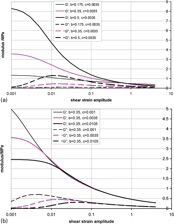
Effect of a parameter b, and b parameter c on elastoplastic dynamic shear moduli A = 0·5 MPa

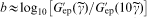
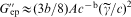
a storage modulus normalised with respect to result obtained after scragging to 10%; b loss modulus normalised with respect to result obtained after scragging to shear strain amplitude of 10%; c effect of scragging strain amplitude on dynamic shear moduli at 1% for EDS16 (regression line is for G″ data force fitted through unity at 10% scragging amplitude); d estimates of b obtained from gradient at strain of 10% of log10 (
) versus log10 (γ)
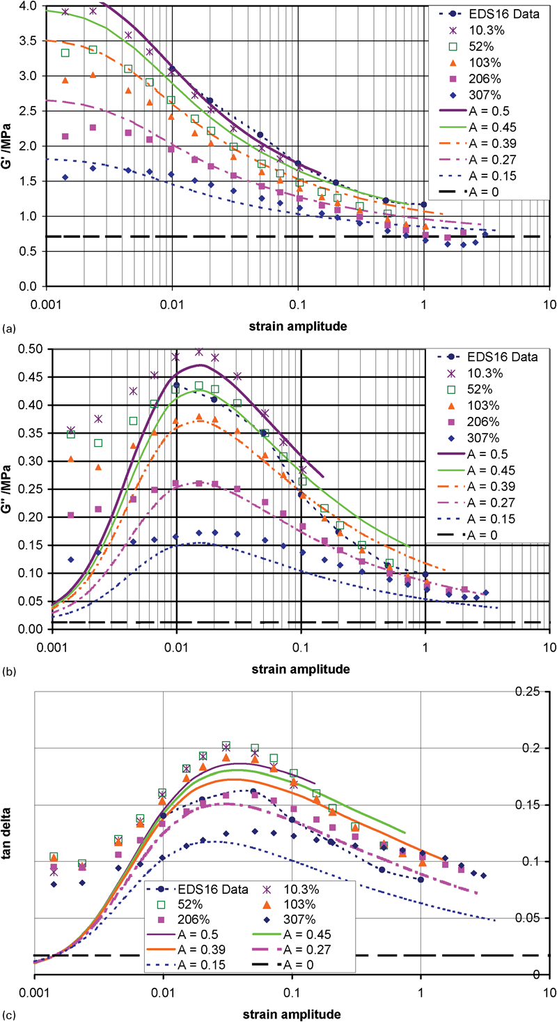
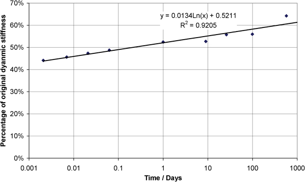
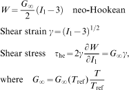
Effects of strain (abscissa) and scragging prestrain (key for symbols) on a storage shear modulus; b loss shear modulus; c loss tangent of EDS16: points, experimental; lines, fits from viscoplastic model (G∞ = 0·593 MPa, H0 = 0·00638, Hm = 0·00089, m = 0·45, A from the G″ trend line of Fig. 4c, b = 0·35 and c = 0·0035)
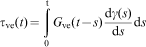
Recovery of original stiffness (1% dynamic strain) over time elapsed since material was tested to ±307% shear strain
Experimental results showing that there is a slow recovery in stiffness are also given, and this effect too may be included in the model.
Viscoplastic model
The model has previously been described in detail8, 9 and is summarised in Fig. 1. It is built on elements evolved in rubber science and technology so that the parameters may connect to physical processes and be minimal in number and maximal in scope to capture the behaviour in a comprehensive manner. Figure 2 shows the hysteresis loops from separate contributions for a particular choice of parameters and their summation to form the total loop.
Hyperelastic contribution – one parameter G∞
The hyperelastic contribution comes from the polymer network and is described by the strain energy function W. The simplest such function can be derived from the statistical theory of rubber elasticity11 and predicts linear behaviour in simple shear
Viscoelastic contribution – one parameter H0 plus m, Hm and aT(T) for fitting to effect of temperature
The viscoelastic contribution comes from the molecular relaxation behaviour,13 and the simplest linear model, based on the Boltzmann superposition principle, is proposed for it. A Prony series discretisation for the relaxation shear modulus G(t), in which the coefficients in the series are not regarded as independent parameters but derived from a small set of basic parameters by a simple equation, has proved useful8, 10

The hysteresis loops predicted by equations (2)–(4) have been calculated for the unfilled rubber matrix, with the stress again boosted by the hydrodynamic factor (1+2·5φ), and are given in Fig. 2b.
Elastoplastic contribution – three parameters A, b and c (plus E for effect of temperature)
This part of the model provides the major contributions to hysteresis for filled rubber and involves a choice of loading function and a set of rules for the subsequent retraction behaviour, spelt out by Ahmadi and Muhr9 but believed to be equivalent to a continuum of elasto-perfectly plastic contributions
 and
and
 and the secant shear modulus Gep(γ) is replaced by the dynamic storage modulus
 .
.
Parameter A represents the elastoplastic contribution to secant shear modulus at
 . Parameter b gives a measure of the steepness of the decline in
 as the shear strain is increased, so that raising b will enhance the elastoplastic modulus contribution for small strains (
 <1) and decrease the contribution at large strain (
 >1). For values of
 >10c, equation (5) implies that
 . Parameter c controls the limiting behaviour as γ→0, in particular the strain at which
 asymptotes to the plateau value [given for the secant value by
 (0) = Ac−b] and the strain at which
 reaches a maximum. For
 , it can be shown that
 . Figure 3a shows the effect of b on
 and
and
 , and Fig. 3b shows the effect of c. The results plotted in these figures were calculated by first generating hysteresis loops from equations (5) and (6) for the chosen parameters and then extracting equivalent viscoelastic parameters
 and
and
 using harmonic analysis.14 The numerical calculations were carried out in an Excel spreadsheet using the trapezium rule; interpretation of fine details in the plots should be viewed with caution. Figure 3a shows that the intersection of the G′–strain amplitude curves for different values of b occurs at a strain amplitude somewhat <1, since the secant stress peak value is rounded off in the harmonic linearisation.
The hysteresis loops calculated from the elastoplastic contributions and the total loops obtained by summing all three contributions are shown in Fig. 2c and d respectively.
Fits to filled natural rubber
The values for the parameters used to generate the hysteresis loops in Fig. 2 were chosen by Muhr10 to fit the experimental results for published data6 for EDS16 (NR+45 pphr N330). To generate these data, two scragging strains were used: 10% for data up to and including 10% shear strain, and 100% for data up to and including 100% strain. A single testpiece was used, but the room temperature measurements were performed first and in the order of ascending strain for strains above 10%, so that for them the test and scragging strains are the same for strains above 10%. Together with the Williams–Landel–Ferry equation, the values for the parameters given in Fig. 2 provided fits10 to dynamic properties for frequencies of 0·1–15 Hz, temperatures of −25 to +100°C and shear strain amplitudes of 1–100%. Similar materials with 0, 15 and 30 pphr N330 were also fitted to the model,10 and it was found that this could be performed by adjusting the elastoplastic modulus A only, in addition to the filler volume fraction used to adjust the hydrodynamic factor that is given, not fitted. In this paper, the fits are extended to include the effect of scragging, as determined for EDS16.7 The primary interest is the effect of quite large scragging strain amplitudes (>10%), representative of the upper limit for strains seen in service, on the dynamic properties at small strains (<10%) typical of normal vibratory excitations for many rubber components, being the conditions in which the component is designed to function for most of the time.
Figure 4a and b shows the experimental data7 plotted as the ratio of storage and loss moduli respectively, for seven different scragging strains, to the modulus measured at the same test strain but for a reference scragging to 10% strain.
For the storage modulus (Fig. 4a), it is evident that in the range of 3–10%, there is relatively little effect of test strain on the ratios, but below 3%, the effect becomes progressively more pronounced. Figure 4b shows a rather different behaviour for the loss modulus, with a smaller effect on the modulus ratios for test strains <3%. It also shows less effect of scragging strains below 10%. Note that for scragging to 10% and above, however, there is quite good agreement between the smallest strain results for modulus ratios in Fig. 4a and b. According to equations (5) and (6), the elastoplastic contribution to G″ falls to zero in the small strain limit, an observation not inconsistent with the somewhat erratic behaviour of the modulus ratio in Fig. 4b at small test strains.
The plots in Fig. 4b are approximately horizontal lines, leading to the following simplifying assumption
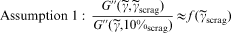
Figure 4c shows factors by which the storage G′ and loss G″ moduli, measured at 1% strain and relative to the results for 10% scragging strain, are reduced as a function of scragging strain.7
In Fig. 4c, the decrease in G″ with increasing scragging amplitude is more pronounced for scragging strains larger than 50% than that for G′. Since
 makes the overwhelming contribution to G″, whereas
 ,
,
 and
and
 all make significant contributions to G′, it appears that scragging acts primarily on the EP contribution. This is also qualitatively consistent with the curvature at test strains below 3% noted in the plots of Fig. 4a: the elastoplastic contribution in the model is solely responsible for the effect of test strain amplitude on G′, so if scragging predominantly affects the elastoplastic branch, then the modulus ratio would be reduced the most at low strains when the elastoplastic contribution is greatest. Together with the interests of simplicity, this observation motivates the following assumption:
Assumption 2: scragging only affects EP contribution
Figure 4d shows estimates of b taken to be
 , where G′ is the experimental result,
 is an estimated value for the purposes of modelling (independent of strain and, by Assumption 2, also independent of scragging strain) and
 has been taken as 10%, with Δ indicating that a secant slope has been calculated from the nearest data points above and below
 = 10. Guidance has been taken from Muhr10 for a fit to the original EDS16 data, for which
 = 0·7097 and b = 0·35. The value of
 was constructed by adding the hyperelastic contribution G∞ = 0·4 MPa and the viscolelastic contribution G′ve = 0.0786 MPa from H0 = 0·0043 MPa for the unfilled matrix rubber and multiplying by a hydrodynamic ‘correction’ factor12 of 1·483 calculated as 1+2·5φ. It appears that the current data have fair consistency with these values of
 and b for all scragging strains, though it could be argued from Fig. 4d that an increase in b to 0·43 and a decrease in
 to 0·66 would be better for scragging strains in the range of 20–300%.
A final simplifying assumption is now proposed:
Assumption 3: scragging affects EP modulus A but not parameters b and c
This leaves only A as a fitting parameter if the values for G∞, H0, Hm, m, b and c from the fit to the original EDS data,6 as given in Fig. 2d are retained. That dataset, however, did not enable a critical fit for c, since the minimum strain amplitude was 1%, whereas c predominantly affects the stress for lower strains (see Fig. 3b).
Figure 5 shows Kingston's data7 for G′, G″ and tan δ respectively after selected scragging strains, together with the original EDS16 data and the simulations from the model. The lines for A = 0 give the hyperviscoelastic contributions according to the model, confirming that these are more significant for G′ than for G″ or tan δ, except at the lowest strains. Figure 5b shows that the strain amplitude at which G″ peaks depends little on the scragging strain, consistent with no change to c (see Fig. 3) and hence Assumption 3. This strain amplitude is, though ∼1·5%, consistent with a smaller value of c (i.e. 0·0035) than used in the fit to the original data (i.e. 0·006). An attempt was made to adjust A to an appropriate value for each level of scragging while keeping c fixed at 0·0035 and the remaining five parameters fixed at the original values.
The values for A were estimated by multiplying the original EDS16 value of 0·5 MPa by factors calculated according to the trend line shown for
 in Fig. 4c. To maintain the time domain and three-dimensional character of the model, it is necessary to define the behaviour for load histories other than steady state shear cycles for which A has been so fitted. As a working rule, the following damage law is tentatively proposed

 for a simple shear strain of γmax, and A0·1 is the value of A for
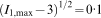 . Thus, A would fall continuously during straining beyond a previous value for I1,max but remain constant for retraction or subsequent straining below the new value of I1,max. Equation (7) would need to be modified for applications for which |γmax| <0·1 or |γmax| >4·4, but this is left for future work.
Figure 5a and b compares Kingston's data to equivalent linear harmonic storage and loss moduli respectively calculated from hysteresis loops generated by the model, fitted as described above (i.e. same parameters as in Fig. 2d, except c = 0·0035 and A = 1·023–0·2325γscrag). Note that the same hysteresis loops are used to generate the model predictions in Fig. 5.
The original EDS16 data are included in the figures. This data agrees well with the present results for G′ up to 10% but gives substantially higher values at 50 and 100%. Conversely, for G″, the original data are lower than the data from Kingston6 for strains below 10% and in quite good agreement above.
Recovery
Figure 6 illustrates the recovery of the initial stiffness at 1% dynamic strain over time. While the recovery is significant, the rubber is not expected to recover its initial unscragged properties. The linear regression line in Fig. 6 would imply that after ∼3×10¹⁵ days, the dynamic shear modulus will rise above the initial modulus, but clearly before then, the rubber would have undergone significant chemical change and hence changes in properties, due to aging. In terms of the model presented above, it would appear that scragging reduces the elastoplastic coefficient A, so it would be straightforward to add a recovery of the magnitude of A, after scragging, that is linear with log time for moderately long recovery periods. Aging of the rubber matrix will result in changes to the hyperelastic and viscoelastic contributions.
It is beyond the scope of the present paper to consider the softening caused by strain history during the recovery period.
Discussion
The G′ data, for 1–10% strain, and the G″ data, for 10–100% strain, presented in Fig. 5, show good agreement between those of Kingston7 and of EDS166 despite the differences in mixer and operators to prepare the material and equipment and operators to measure the dynamic properties. This provides confidence that the values of the fitting parameters chosen by Muhr10 remain useful for estimating the properties of future batches of this material and justifies their application to Kingston's data in this paper with the only adjustment made being that to c. In consequence, focus on the effect of scragging has been maintained. Since, according to the model and the particular choice of parameters, G″ is almost entirely controlled by the elastoplastic contribution for this material, as seen by comparing the line for A = 0 with the experimental data, the effect of scragging on the elastoplastic parameters has been quantified through its effect on G″. Making the simplifying assumptions that b and c are not affected by scragging, the remaining elastoplastic parameter A can be fitted from a plot of G″, at any test strain amplitude, versus the scragging strain amplitude. From this plot (Fig. 4c), it is apparent that a linear regression fit is reasonably good, so that A may be reasonably well approximated by a reduction proportional to the scragging strain. This observation, together with the adjustment to c to give reasonable agreement to the strain amplitude at which G″ is maximum, completes the effort of fitting parameters in this paper. Following this point, attention can be focused onto Fig. 5, where the overall fit of model and experimental data is exposed. First, it is revealed that the agreement between the original EDS16 data6 and that of Kingston7 is much less good for G″ (and tan δ) at low strains than for G′. However, this poorer agreement is relative, and, in absolute terms, the discrepancy is not so dissimilar, when it is appreciated that G″ is an order of magnitude smaller than G′. Thus, part of the poorer apparent fit between the model and G″ or tan δ data than for G′ data may be tentatively attributed to the greater relative experimental uncertainty in the loss data.
Such uncertainty probably cannot explain the much higher G″ values than predicted by the model for the lowest strain amplitudes (<1%). It would appear that for such strains, the filler induced enhancement of G′, and in particular its tendency towards a plateau value at low strain, is not coupled to G″ in the way described by the elastoplastic branch of the model. Similarly, scragging amplitudes less than ∼10% cause much higher softening for G′ than expected from the regression fit to the G″ data, again pointing to the weaker coupling between G′ and G″ at low strain. It is interesting to note that, for small strains, tan δ is not as sensitive as the moduli to scragging at amplitudes of 10% and above and is far higher than the value expected from hyperviscoelasticity. It would appear that the high experimental values of G″ for γ<c point to a dissipative mechanism that is neither related to breakdown and recovery of a filler structure during cycling (since that would imply a negative gradient for G′ versus strain amplitude) nor to the normal viscoelasticity of the rubber matrix. Instead, it could be due to a modification of the viscoelasticity of such matrix rubber as is exposed to extremes of strain amplification and/or proximity to the filler surface.
At strain amplitudes >100%, Fig. 5 shows discrepancies between model and experiments for all three properties. Such discrepancies are less striking than those at low strain but could point to the stress softening of the matrix rubber. High strains also raise questions regarding the experimental technique, the finite strain capability of the hyperviscoelastic and elastoplastic models and the possibility of strain crystallisation of the rubber, which is beyond the capability of the model. There is probably also less practical need to devise a model with very high strain capability so this issue is not addressed here.
In summary, a time domain viscoplastic model8–10 has been extended to include the effect of scragging, which appears to act only or at least predominantly on the elastoplastic contribution associated with the filler. It is found to work reasonably well for test strain amplitudes between 1 and 100% shear strain and scragging strains of 10% and above. The values of the parameters fitted to earlier data for the same formulation fitted the current equivalent data moderately well after adjustment of just one parameter, primarily to modify the fit beyond the range of strain amplitudes used in earlier tests. The model is commended for practical use. It may also serve towards the interpretation of the behaviour of rubber, but as it is not expected to capture all details of the behaviour or coupling of the contributions, it must be borne in mind that such interpretations are constrained by the artificial limitations of the model.
Conclusions
Increasing the scragging shear strain up to 300%, applied to natural rubber filled with 45 pphr N330 carbon black, resulted in a continuous fall in the dynamic shear moduli at lower strains, with no evidence of a lower limit being reached. Slow recovery in storage modulus occurred over time.
The proposed time domain viscoplastic model gives a useful approximation to the data for test strains ranging from 1 to 100% and scragging strains >10%. The effects of filler loading,10 scragging strain amplitude and recovery may all be accommodated by adjusting only one parameter, i.e. the elastoplastic shear modulus A at ∼100% strain.
The basic model has five parameters to describe the stress–strain behaviour in the absence of temperature variation and stress softening. The effect of scragging can be described by a one-parameter damage model corresponding to the reduction in elastoplastic modulus A with scragging strain. An additional parameter could be used for the recovery in A per tenfold increase in time elapsed since scragging to the largest strain.
The fit to loss modulus G″, involving no extra parameters, is relatively poor compared to that for storage modulus G′, pointing to a different mechanism contributing damping at very low strains (<1%). Some improvement might be possible by optimising the values for the EP parameters or the choice of elastoplastic function.
Footnotes
Acknowledgements
Thanks are due to H. R. Ahmadi for discussion of the work and checking the manuscript.