A Framework and Case Study for Earthquake Vulnerability Assessment of Incrementally Expanding Buildings

Abstract

This study proposes a framework for incorporating time-dependent fragility into large-scale risk assessment models, focusing on incremental building expansion as a significant driver of changes in vulnerability. In rapidly urbanizing areas in developing countries, the pay-as-you-go process of informal building construction and staged expansion is the de facto pattern of growth. While there is a common understanding that such expansions increase the earthquake vulnerability of buildings, this study proposes a framework to model and quantify this increase. Vulnerability curves are developed through incremental dynamic structural analysis for common building expansion typologies. Building expansions are modeled as Markov chain processes and used to simulate stochastic expansion sequences over a building's lifetime. The model is then used to simulate a hypothetical neighborhood in the Kathmandu valley area to understand neighborhood-level risk over time. The study provides a new methodology to analyze changing seismic risk over time, driven by any building modification that impacts the building's vulnerability (incremental expansion, deterioration, retrofit, etc.).

Introduction

The year 2008 marked a significant threshold in the history of human settlement, when for the first time urban dwellers outnumbered rural dwellers. This dramatic transformation has been described as “one of the most powerful, irreversible, and visible anthropogenic forces on Earth” (Laumann 2005). By 2030, the global population will reach 9 billion, of which 60% will reside in cities (United Nations 2005). Most of this urban growth will occur in cities in developing countries (United Nations 2005), where the pay-as-you-go process of informal building expansion is the de facto pattern of growth. Households start with simple one- or two-story shelters, which over time—and given sufficient resources—are transformed incrementally into multistory homes and rental units, as can be seen in Figure 1. The concept of a “static” building—designed by an architect or engineer, constructed according to construction blueprints, and subsequently remaining as such for its lifetime—is the exception rather than the norm. Buildings are not static, but evolve over time, reflecting patterns of cash flow, family expansions, investments in home businesses, and other factors. While structural building types and construction materials vary widely, the basic incremental building process is ubiquitous in developing countries across the world. This bottom-up approach to city building has received increasing attention by researchers, as it has been one of the only ways for cities to respond to their incredible housing and infrastructure needs (Ferguson and Smets 2010).

Figure 1.

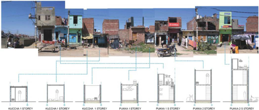
Diagram of the process of incremental building construction typical of cities throughout the world. Source: King 2011.

Despite the fact that buildings are rarely static, one of the assumptions implicit in current risk assessment models is that vulnerability is constant over time. The current study proposes a framework for incorporating time-dependent fragility into large-scale risk assessment models, focusing on incremental building expansion as a significant driver of increase in vulnerability. The increase in vulnerability linked with building expansion is expected since the majority of such building expansions are not designed anticipating the loads of additional stories, nor are they strengthened in the expansion process. While the greater vulnerability of expanded buildings is known, this study is the first attempt at quantifying the increases in earthquake vulnerability linked to common building expansions. It further looks at a hypothetical case study in Kathmandu, Nepal, to demonstrate the broader risk impact as young neighborhoods (mainly single-story buildings) grow and densify over time (mainly multistory buildings).

The primary contribution of the paper is in providing a methodological framework for evaluating time-dependent seismic risk linked with incremental building expansion. The case study serves as an example and as a proof of concept rather than a prediction of actual risk. While the study focuses on building expansion, the framework could equally be used to model other drivers of changing vulnerability such as deterioration and retrofit. Finally, the study hints at possible nontraditional approaches to reducing earthquake risk, such as simple policies limiting building expansions or linking expansions with strengthening.

Incrementally Expanding Building Morphologies

In dense urban environments, ground-level building footprints are typically constrained by neighboring buildings. Building expansions therefore consist of vertical extensions (additional stories) and horizontal extensions (additional stories cantilevered above sidewalks or streets). These two basic extensions can be combined to form a variety of building morphologies.

For the purposes of this study, a standard building layout was developed for a typical residential building. This study focuses specifically on concrete frame buildings with masonry infill, which represent a very common construction type in developing countries around the world. It further focuses on buildings that expand to no more than three stories. The catalog of common expansion morphologies presented in Figure 2 includes 9 building morphologies, from which numerous evolutionary building sequences are possible. In order to keep the study both general and realistic, building morphologies were developed that are emblematic of real buildings found in Kathmandu, Nepal, as pictured in Figure 3.

Figure 2.

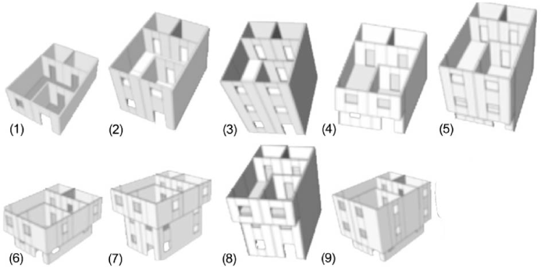
Ten common building morphologies.

Figure 3.

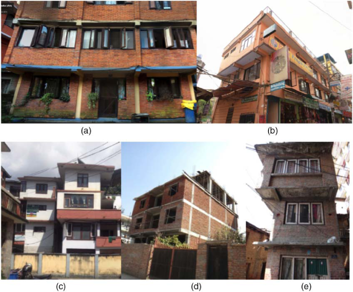
Buildings in Kathmandu, Nepal, showing typical incrementally expanded building morphologies. Source: Google Street View (a, b, and c); Anne Sanquini (d and e).

Building Vulnerability Modeling

The earthquake vulnerability of buildings is defined by fragility curves. These describe the relationships between the intensity of earthquake ground motion and the probability of experiencing or exceeding a particular level of damage. They can be developed (1) analytically, based on structural modeling and response simulation (Singhal and Kiremidjian 1996, Rossetto and Elnashai 2005, Ibarra and Krawinkler 2005, Lallemant et al. 2015), (2) empirically, based on statistical analysis of post-earthquake damage assessment data (Laumann 2005, Colombi et al. 2008, Sabetta et al. 1998, Noh et al. 2014), or (3) heuristically, based on expert opinion (United Nations 2005, Jaiswal et al. 2012, ATC 1985).

In this study, analytical collapse fragility curves were developed for each of the nine building morphologies. Specific structural parameters were defined based on the National Nepalese Building Code document Mandatory Rules of Thumb—Reinforced Concrete Buildings with Masonry Infill (Nepal Department of Urban Development and Building Construction 1994). The collapse performance assessment was conducted using incremental dynamic analysis (IDA) (Singhal and Kiremidjian 1996, Vamvatsikos and Cornell 2002, Rossetto and Elnashai 2005, Ibarra and Krawinkler 2005). Nonlinear dynamic analyses are conducted on a two-dimensional (planar) model developed in OpenSees (Mazzoni et al. 2006) using the 22 far-field ground motion set and scaling method outlined in FEMA P695 (FEMA 2009). Peak ground acceleration (PGA) is used as the ground motion intensity measure. The overall analysis approach is based on the methodology developed by Burton and Deierlein for simulating the seismic collapse of nonductile reinforced concrete frame buildings with infill (Burton and Deierlein 2014).

Collapse fragility curves are developed based on the IDA results and fit using a generalized linear model with the probit link function using log(IM) as the independent variable (Lallemant et al. 2015). This is identical to fitting a lognormal CDF curve by maximum likelihood estimation. The generalized linear model formulation of fragility curves is described by Equation 1.

P (c o l l a p s e | I M) = Φ (α + β \log (I M))

(1)

Sample fragility curves for a specific building sequence are shown in Figure 4, and fragility curves for all building state typologies are given in Figure 5. The parameters α and β of the fragility curves are shown in Table 1.

Figure 4.

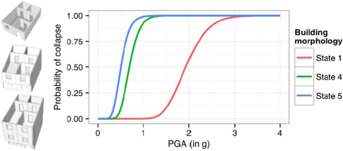
Sample building sequence and associated changes in vulnerability curve. PGA = peak ground acceleration; g = acceleration of gravity.

Figure 5.

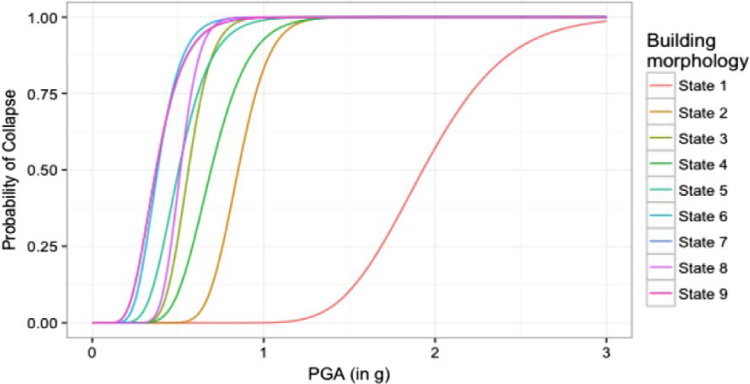
Fragility curves for all building stages.

Table 1

Fragility curve parameters for all building state typologies used to define fragility curves using Equation 1

Typology	1	2	3	4	5	6	7	8	9
α	-3.28	0.95	2.98	1.45	2.31	3.32	2.83	3.89	2.85
β	5.00	5.92	5.15	3.95	3.38	3.44	2.86	5.85	2.87

Rate of Building Expansion

Building expansion over time occurs as a discrete process, often linked to capital flows and/or family expansion. For any given time increment, a building may expand or may stay in its current state. In order to simulate this, a Markov chain process model is developed. Markov chains are used to simulate mathematical systems that transition from one state to another in state space. These models are “memoryless,” such that the next state is only dependent on the current state, not on the sequence of events that preceded it (Agresti 2002). A transition matrix is used to define the probability of transitioning from any state to another in a given time period. It is described in Equation 2.

P = {\begin{matrix} p_{1, 1} & p_{1, 2} & p_{1, 3} & \dots & p_{1, 9} \\ p_{2, 1} & p_{2, 2} & p_{2, 3} & \dots & p_{2, 9} \\ p_{3, 1} & p_{3, 2} & p_{3, 3} & \dots & p_{3, 9} \\ ⋮ & ⋮ & ⋮ & ⋱ & ⋮ \\ p_{9, 1} & p_{9, 2} & p_{9, 3} & \dots & p_{9, 9} \end{matrix}} = {\begin{matrix} p_{1, 1} & p_{1, 2} & p_{1, 3} & \dots & p_{1, 9} \\ 0 & p_{2, 2} & p_{2, 3} & \dots & p_{2, 9} \\ 0 & 0 & 1 & 0 & 0 \\ ⋮ & ⋮ & ⋮ & ⋱ & ⋮ \\ 0 & 0 & \dots & \dots & p_{9, 9} \end{matrix}}

(2)

where p_1,2 is the probability of transitioning from the first to the second building morphology.

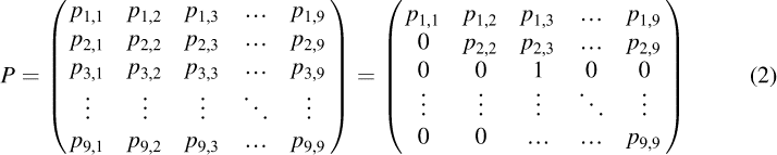
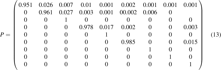
The transition matrix simplifies, as shown in Equation 2, because it is assumed that buildings do not transition to lower states (removing an extension), and because some states are “absorbing states,” which once entered cannot be left (since we assume no expansion beyond three stories). Therefore, all lower triangle terms reduce to probability zero and all terms in which the current state corresponds to a three-story building have probability one. All other terms can be calibrated to context-specific transition rates based on observations of buildings over time. The data required to calibrate the transition probability matrix for buildings in Kathmandu were unavailable, and missing terms were therefore assumed and checked for reasonable outcomes of building state distribution after 10, 25, and 50 years based on studies by the Global University Consortium on Incremental Housing (Marome and Rittironk 2011, Guerra Sousa 2010). In future studies, transition probability rates will be obtainable based on statistics of building state distribution over time. Continuous monitoring of such data is unlikely to ever be common, but if the building state distribution is known at two snapshots in time, the transition rates can be estimated even without knowing the specific trajectory from start to ending state. The maximum likelihood estimation method can be used to estimate unknown transition probability parameters most likely to lead to the observed outcome. Other optimization methods have been developed to calibrate transition probability matrices (Welton and Ades 2016, Baik et al. 2006). For any given starting state, an expansion sequence can be simulated and tracked over time, as demonstrated in Figure 6.

Figure 6.

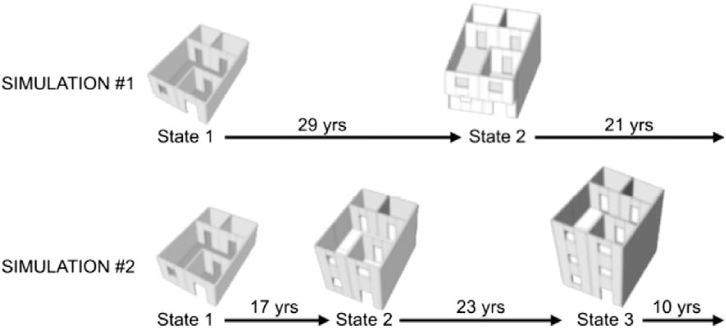
Sample simulation of stochastic building expansion over time based on Markov chain process.

While not modeled explicitly, the rate of building expansion could be spatially correlated and such correlation included in the model. If the data of such correlation existed, it could be accounted for by spatially heterogeneous transition probability matrices, whose parameters are spatially correlated random variables rather than constants (Lallemant 2015).

Markov chain simulations provide a simple method to map the distribution of building states over time. This is done through iterative sampling of the state space weighted by the appropriate row of the transition probability matrix. By simulating thousands of such chains, Figure 7 shows the distribution of building states after 10, 25, and 50 years, assuming that 75% of buildings start in State 1 (single story) and 25% start in State 2 (two story).

Figure 7.

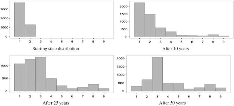
Distribution of buildings states after 10, 25, and 50 years, based on simulation of incremental building expansion on 5,000 buildings; starting distribution is 75% in State 1 and 25% in State 2.

Alternatively, we can calculate the n-step transition probability of the Markov chain, which describes P(X_n = j | X₀ = i), the probability of being in state j after n steps given a starting state i. Also denoted $p_{i j}^{(n)}$ , this is calculated as the sum of the probabilities of all paths from i to j in n steps. As long as the probability distribution on the state space of the Markov chain is discrete and the Markov chain is homogeneous (not changing in time), the Chapman-Kolmogorov equations can be used to demonstrate that this result is equal to multiplying the transition matrix by itself n times: P⁽ⁿ⁾ = Pⁿ.

For an arbitrary square matrix, this operation is complex, but can be significantly simplified through eigendecomposition. In our case, the square transition matrix P can be factorized as P = EΛE⁻¹, where E is a square matrix whose ith column is the eigenvector e_i of the transition matrix P, and whose Λ is the diagonal matrix constructed from the corresponding eigenvalues. It follows that

P^{n} = {(E Λ E^{- 1})}^{n} = (E Λ E^{- 1}) (E Λ E^{- 1}) \dots (E Λ E^{- 1}) = E Λ^{n} E^{- 1}

(3)

The nth power of diagonal matrix Λ is much simpler to find than the nth power of the original transition matrix P.

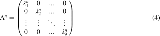
Λ^{n} = (\begin{matrix} λ_{1}^{n} & 0 & \dots & 0 \\ 0 & λ_{2}^{n} & \dots & 0 \\ ⋮ & ⋮ & ⋱ & ⋮ \\ 0 & 0 & \dots & λ_{9}^{n} \end{matrix})

(4)

Also, for any group of buildings with a distribution of typologies described by a normalized vector d₀, the expected distribution D_n after n steps can be described as

E (D_{n} | D_{0} = d_{0}) = d_{0} P^{n} = d_{0} E Λ^{n} E^{- 1}

(5)

Equation 5 can therefore be used to calculate the expected distribution of building typologies after t years (replacing n steps by t years). Figure 8 shows this distribution as a function of time, given a starting distribution of building typologies of 75% in State 1 and 25% in State 2.

Figure 8.

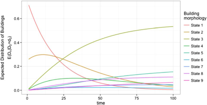
Building typology distribution over time, assuming all buildings start in State 1.

As can be observed from Figure 8, the probability of being in a transient state (any building typology with a nonzero probability of transitioning to another state) goes to zero with time. Eventually all buildings are in an absorbing state (one of the six three-story building typologies).

Collapse Probability

The rate of collapse of a building over a period t can be computed by integrating its collapse fragility curve over the hazard function, following Equation 6.

λ_{C o l l a p s e} (t) = t \int_{I M_{\min}}^{I M_{\max}} P (C o l l a p s e | I M = i m) | d λ_{I M} (i m) |

(6)

where t is the time interval of interest (typically lifetime or annual), λ_Collapse is the expected rate of collapse over that time, P(Collapse | IM = im) is the probability of collapse given IM = im (the fragility curve), and λ_IM(x) is the mean annual frequency of IM exceeding im (the hazard curve).

As described previously, incrementally expanding buildings change fragility with each increment. Hence the collapse rate needs to reflect the time dependence of fragility. Equation 6 therefore becomes

\begin{matrix} λ_{C o l l a p s e} (t) = \sum_{S_{i} = 1}^{9} \int_{0}^{t} \int_{I M_{\min}}^{I M_{\max}} P (C o l l a p s e | I M = i m, S = s_{i}) \\ P (S_{n} = s_{i} | S_{0} = s_{0}) | d λ_{I M} (i m) | d n \end{matrix}

(7)

where P(Collapse|IM = im, S = s_i) is the fragility curve for building typology i, and P(S_n = s_i | S₀ = s₀) is the probability of being in state s_i after n steps (at time t) given a starting state s₀. The calculation is summed over all possible building states s_i.

Equation 7 can be re-written as

\begin{matrix} λ_{C o l l a p s e} (t) = \sum_{S_{i} = 1}^{9} [\int_{0}^{t} P (S_{n} = s_{i} | S_{0} = s_{0}) d n \\ \int_{I M_{\min}}^{I M_{\max}} P (C o l l a p s e | I M = i m, S = s_{i}) | d λ_{I M} (i m) |] \end{matrix}

(8)

We note that P(S_n = s_i | S₀ = s₀) was described in matrix form by Equation 5 and that

\int_{I M_{\min}}^{I M_{\max}} P (C o l l a p s e | I M = i m, S = s_{i}) | d λ_{I M} (i m) |

is the annual collapse rate for each building typology i. We denote the vector of these annual collapse rates Λ_CR = [λ_{CR
₁}, λ_{CR
₂}, …, λ_{CR
₉}. Equation 8 can then be rewritten in matrix form as

\begin{matrix} λ_{C o l l a p s e} (t) = \int_{0}^{t} P^{n} d n Λ_{C R} \\ = \int_{0}^{t} E Λ^{n} E^{- 1} d n Λ_{C R} \\ = E [\int_{0}^{t} Λ^{n} d n] E^{- 1} Λ_{C R} \end{matrix}

(9)

We also note that the term

\int_{I M_{\min}}^{I M_{\max}} P (C o l l a p s e | I M = i m, S = s_{i}) | d λ_{I M} (i m) |

defines the expected amount of time spent in each state in a period of t years. This calculation is therefore the amount of time in each state multiplied by the collapse rate for that building typology, summed up for every state.

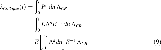
The diagonalization of the transition matrix described in Equation 5 enables us to solve the integration as a matrix of integrals of the eigenvalues to the nth power.

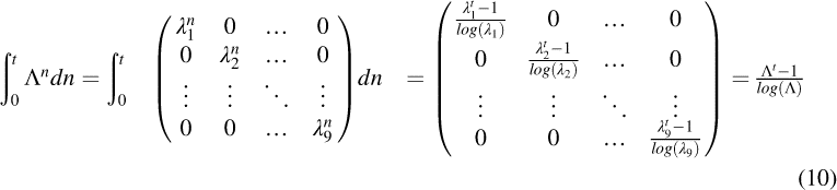
\int_{0}^{t} Λ^{n} d n = \int_{0}^{t} (\begin{matrix} λ_{1}^{n} & 0 & \dots & 0 \\ 0 & λ_{2}^{n} & \dots & 0 \\ ⋮ & ⋮ & ⋱ & ⋮ \\ 0 & 0 & \dots & λ_{9}^{n} \end{matrix}) d n = (\begin{matrix} \frac{λ_{1}^{t} - 1}{\log (λ_{1})} & 0 & \dots & 0 \\ 0 & \frac{λ_{2}^{t} - 1}{\log (λ_{2})} & \dots & 0 \\ ⋮ & ⋮ & ⋱ & ⋮ \\ 0 & 0 & \dots & \frac{λ_{9}^{t} - 1}{\log (λ_{9})} \end{matrix}) = \frac{Λ^{t} - 1}{\log (Λ)}

(10)

Equations 9 and 10 can be combined as

λ_{C o l l a p s e} (t) = E [\frac{Λ^{t} - 1}{\log (Λ)}] E^{- 1} Λ_{C R}

(11)

If an eigenvalue λ_i equals or very closely approximates 1, then the $\frac{1}{\log (λ_{i})}$ term is undefined (since log(1) = 0). However, $\int_{0}^{t} 1^{n} d n = t$ , which can be used for that specific entry in the matrix of Equation 10.

The result of Equation 11 is a vector describing for each starting state the rate of collapse over the period t. If, rather than a single building with a given starting state, we are instead interested in the rate of collapse for a portfolio of buildings with various starting states, we add to Equation 11 the normalized vector of starting distribution of building states for that portfolio, as was done in Equation 5.

λ_{C o l l a p s e} (t, D_{0} = d_{0}) = d_{0} E [\frac{Λ^{t} - 1}{\log (Λ)}] E^{- 1} Λ_{C R}

(12)

Applications

Two main applications are developed in this section. The first is to compute the lifetime rate of collapse of a single building in Kathmandu, Nepal, reflecting its potential expansion over time. The second application is to compute the predicted collapse rate of an entire neighborhood in the Kathmandu Valley for a specific earthquake scenario.

Probabilistic Seismic Hazard of Kathmandu

All of Nepal is exposed to significant earthquake hazard resulting from the convergence of the Indian tectonic plate with the Eurasian plate, which also drives the uplift of the Himalayan mountain range. The April 2015 M_w 7.8 earthquake in Nepal is a reminder of the high seismicity of the region. The earthquake is estimated to have resulted in nearly 10,000 fatalities and the collapse of approximately 500,000 buildings (Government of Nepal 2015). During the 1934 Great Nepal-Bihar Earthquake (M_w 8.2), almost all buildings collapsed in Kathmandu, Bhaktapur, and Patan and casualties were estimated to be as high as 12,000. Other major earthquakes have occurred in 1897, 1905, 1934, and 1950.

It is estimated that at least four events of 8.2 < M_w < 8.6 would need to occur in the Himalayas to release the tectonic strain accumulated by the plate collision over recent centuries (Bilham and Ambraseys 2005). It is therefore of note that the 25 April M_w 7.8 earthquake and the 12 May M_w 7.3 aftershock have not significantly reduced the accumulated energy in the plate boundary. In other words, large earthquake events are still expected.

A probabilistic seismic hazard model was developed for Kathmandu based on a source model developed by Shrestha in 2014 (Shrestha 2014). This model assumes ten independent sources contributing to the seismic hazard in the Kathmandu Valley. The probabilistic hazard model developed by Shrestha was updated using Boore and Atkinson 2008 ground motion prediction relationship (Boore and Atkinson 2008). The resulting annual PGA hazard curve is shown in Figure 9.

Figure 9.

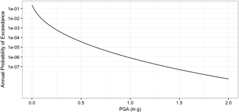
Hazard Curve for Kathmandu.

Lifetime Probability of Collapse of a Building Expanding over Time

We are interested in the lifetime probability of collapse of a building that starts in State 1 but is expected to expand following transition probabilities as shown in Equation 13 and corresponding to the building state typologies shown in Figure 2.

P = (\begin{matrix} 0.951 & 0.026 & 0.007 & 0.01 & 0.001 & 0.002 & 0.001 & 0.001 & 0.001 \\ 0 & 0.961 & 0.027 & 0.003 & 0.001 & 00.002 & 0.006 & 0 \\ 0 & 0 & 1 & 0 & 0 & 0 & 0 & 0 & 0 \\ 0 & 0 & 0 & 0.978 & 0.017 & 0.002 & 0 & 0 & 0.003 \\ 0 & 0 & 0 & 0 & 1 & 0 & 0 & 0 & 0 \\ 0 & 0 & 0 & 0 & 0 & 0.985 & 0 & 0 & 0.015 \\ 0 & 0 & 0 & 0 & 0 & 0 & 1 & 0 & 0 \\ 0 & 0 & 0 & 0 & 0 & 0 & 0 & 1 & 0 \\ 0 & 0 & 0 & 0 & 0 & 0 & 0 & 0 & 1 \end{matrix})

(13)

Combining the hazard curve (Figure 9) and the fragility curves (Figure 5), we can calculate the 50-year collapse rate of buildings in each possible state assuming that they do not evolve.

\begin{matrix} \int_{0}^{50} Λ_{C R} d t = 50 \times [\begin{matrix} λ_{C R_{1}} \\ λ_{C R_{2}} \\ ⋮ \\ λ_{C R_{9}} \end{matrix}] = 50 \times [\begin{matrix} \int P (C o l l a p s e | I M = i m, D = d_{1}) | d λ_{I M} (i m) | \\ \int P (C o l l a p s e | I M = i m, D = d_{2}) | d λ_{I M} (i m) | \\ ⋮ \\ \int P (C o l l a p s e | I M = i m, D = d_{9}) | d λ_{I M} (i m) | \end{matrix}] \\ = 50 \times [\begin{matrix} 4.72 \times 10^{- 9} \\ 4.87 \times 10^{- 7} \\ 3.61 \times 10^{- 6} \\ 1.82 \times 10^{- 6} \\ 7.67 \times 10^{- 6} \\ 1.98 e \times 10^{- 5} \\ 2.50 \times 10^{- 5} \\ 4.85 \times 10^{- 6} \\ 2.52 \times 10^{- 5} \end{matrix}] = [\begin{matrix} 2.36 \times 10^{- 7} \\ 2.43 \times 10^{- 5} \\ 1.80 \times 10^{- 4} \\ 9.11 \times 10^{- 5} \\ 3.83 \times 10^{- 4} \\ 9.90 \times 10^{- 4} \\ 1.25 \times 10^{- 3} \\ 2.42 \times 10^{- 4} \\ 1.26 \times 10^{- 3} \end{matrix}] \end{matrix}

(14)

We can then use eigendecomposition of the transition matrix to obtain the eigenvectors E and the diagonalized eigenvalue matrix Λ, which we plug into Equation 11 to get the 50-year collapse rate of buildings assuming they do evolve and expand over time. The resulting vector shows the 50-year collapse rate of buildings for each starting state.

λ_{C o l l a p s e} (50) = E [\frac{Λ^{50} - 1}{\log (Λ)}] E^{- 1} Λ_{C R} = [\begin{matrix} 1.60 \times 10^{- 4} \\ 1.55 \times 10^{- 4} \\ 1.81 \times 10^{- 4} \\ 2.79 \times 10^{- 4} \\ 3.84 \times 10^{- 4} \\ 1.07 \times 10^{- 3} \\ 1.25 \times 10^{- 3} \\ 2.43 \times 10^{- 4} \\ 1.26 \times 10^{- 3} \end{matrix}]

(15)

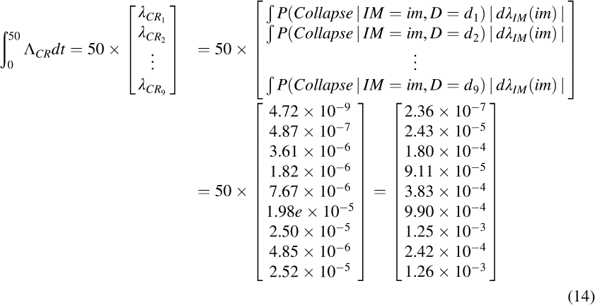
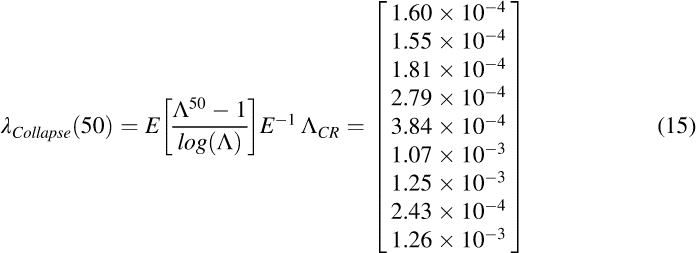
Comparing the results of Equations 14 and 15 shows that the evolving buildings have much higher rates of collapse. Assuming that buildings will stay in their original state throughout their lifetime can lead to significantly underestimating their seismic risk. As is clear from the fragility curves of Figure 5, unless designed at the outset with extra capacity for future expansions, the additional inertial load and load-path discontinuities resulting from these expansions significantly increase buildings’ vulnerability to earthquakes.

Portfolio Risk from Scenario Earthquake

Earthquake scenarios can be used to demonstrate the impact of a potential scenario event on a building, neighborhood, or city. A reproduction of the 1934 Great Nepal-Bihar Earthquake was chosen for this scenario. Spatially correlated earthquake ground motion intensity fields were simulated, reflecting the fact that shaking at sites close to each other is expected to be similar in intensity (Jayaram and Baker 2009). This approach was used to investigate the predicted loss for a portfolio of buildings evolving over time, based on the same baseline earthquake scenario.

In order to demonstrate the impact of incremental expansion on vulnerability over time at a community scale, a hypothetical neighborhood was created consisting of 100 buildings on the outskirts of Kathmandu City. It is a “young” neighborhood, with all buildings in either State 1 or State 2. The growth of this neighborhood is simulated over 30 years, and the collapse rate of buildings in the neighborhood is computed every three years based on the Great Nepal-Bihar Earthquake scenario. The analytical formulation described previously can be used to obtain the expected rates of collapse over time. However, in this application we used a simulation model in order to capture the uncertainty around this expected collapse rate. The uncertainty reflects the uncertainty in ground motion intensity fields as well as the stochastic nature of incremental building expansion.

Figure 10 shows the rate of building collapse over time, driven by the increasing vulnerability of buildings as they expand vertically and horizontally. The figure demonstrates that about 23% percent of buildings could be expected to collapse if the earthquake occurred in 2015, while 56% of buildings would be expected to collapse if it occurred in 2045. This is in large part due to the significant increase in collapse risk as soon as a building extends from one to two stories. The blue bands in the figure indicate that significant uncertainty surrounds these estimates. The trend, however, is clear. Note that the increase in vulnerability is doubly troubling because it is linked with an increase in occupancy as buildings get larger.

Figure 10.

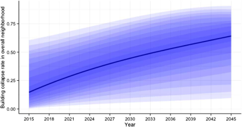
Expected building collapse rate over time in a neighborhood on the outskirts of Kathmandu, based on a reproduction of the 1934 Great Nepal-Bihar Earthquake. Shading reflects uncertainty.

As stated earlier, the results of this incremental risk analysis for a neighborhood in Kathmandu should be used as a methodological demonstration rather than an actual prediction of future seismic risk for that neighborhood. The building vulnerability curves, transition probability matrices, and earthquake source model are all plausible and realistic for Kathmandu, but are based on several assumptions and significant uncertainty.

Conclusion

This study showcases a methodology to model dynamic seismic risk due to changing vulnerability of the built environment over time. While the model is used to demonstrate changing risk due to building expansion, the same methodology could be used to study the impact of improved construction practices, retrofits, and other actions that impact the vulnerability of a building. The specific focus on building expansion stems from a concern for its impact on increasing seismic risk which is currently not accounted for in models that assume that buildings are static in time. Young urban settlements grow through the informal expansions of individual buildings. In many parts of the world, including the fast-growing urban centers of developing countries, these informal expansions constitute the main process of city building. This study looks at the impact of such a process on the earthquake vulnerability of neighborhoods.

We propose a framework for modeling incrementally expanding buildings as a Markov chain process. Analytical formulations are derived to calculate the expected duration of time a building will be in any state of interest given a starting state as a function of time. This result allows us to calculate the expected rate of collapse over a period t of a building given any starting state. We also use a simulation model for incrementally expanding buildings to efficiently capture the full distribution of collapse risk over time for an entire neighborhood. Overall two main conclusions can be drawn from this study, as described in the following paragraphs.

Driven by informal building expansion, risk increases with time. There is a significant earthquake risk linked with informal building expansion. The risk is easy to overlook for a single building or a short time frame, but given enough time and scaled to entire neighborhoods, the incremental expansion process can profoundly shift earthquake risk. In contexts of limited capacity for enforcement of engineering design standards, controlling building expansions (limits on number of floors and cantilevers) is likely feasible even when detailed engineering inspections are not. Governments should consider policies to control the most dangerous expansions and develop design guidelines for expanding safely. Both of these steps would have significant impact on reducing the future seismic risk of cities.

The change in seismic risk is predictable. The disaster risk of rapidly changing cities is predictable even if uncertainties are large. Probabilistic hazard models can be combined with modern structural analysis tools, building expansion simulations, and other models to gain understanding of the main trends in the disaster risk of cities. As part of efforts to ensure that cities are resilient to future disasters, these tools can serve as the basis for risk-informed urban planning and policy analyses that place urban environments on a trajectory to minimize future risk.

Footnotes

Acknowledgments

This research was partially supported by the National Science Foundation Grant NSF CMMI-106756, by the Shah Family Fellowship, and by the John A. Blume Fellowship.

References

Agresti

2002 Categorical Data Analysis Wiley-Interscience Hoboken, NJ.

Applied Technology Council (ATC) 1985 Earthquake damage evaluation data for California. Technical Report ATC-13 Redwood City, CA.

Baik

H.-S.

Jeong

H. S.

and Abraham

D. M.

2006

Estimating transition probabilities in Markov chain-based deterioration models for management of wastewater systems

Journal of Water Resources Planning and Management 132 15–24.

Bilham

and Ambraseys

2005

Apparent Himalayan slip deficit from the summation of seismic moments for Himalayan earthquakes, 1500–2000

Current Science.

Boore

D. M.

and Atkinson

G. M.

2008

Ground-motion prediction equations for the average horizontal component of PGA, PGV, and 5 and 10.0 s

Earthquake Spectra 24 99–138.

Burton

and Deierlein

2014

Simulation of seismic collapse in nonductile reinforced concrete frame buildings with masonry infills

Journal of Structural Engineering 140 A4014016.

Colombi

Borzi

Crowley

Onida

Meroni

and Pinho

2008

Deriving vulnerability curves using Italian earthquake damage data

Bulletin of Earthquake Engineering 6 485–504.

Federal Emergency Management Agency (FEMA) 2009 Quantification of Building Seismic Performance Factors Report No. FEMA P695, Washington, D.C.

Ferguson

and Smets

2010

Finance for incremental housing: current status and prospects for expansion

Habitat International 34 288–298.

10.

Government of Nepal 2015 Nepal Earthquake 2015 Post Disaster Needs Assessment—Vol. A: Key Findings Kathmandu, Nepal.

11.

Guerra Sousa

2010 From Shacks to Homes—Learning from 40 Years and 30 Recent House Examples Technical Report, Global University Consortium Exploring Incremental Housing Chihuahua, Mexico.

12.

United Nations 2005 World Urbanization Prospects: The 2005 Revision Department of Economic and Social Affairs United Nations, New York.

13.

Ibarra

L. F.

and Krawinkler

2005 Global Collapse of Frame Structures under Seismic Excitations Technical Report, John A. Blume Earthquake Engineering Center Stanford University, Stanford, CA.

14.

Jaiswal

K. S.

Aspinall

and Perkins

2012

Use of expert judgment elicitation to estimate seismic vulnerability of selected building types

Proceedings of the 15th World Conference on Earthquake Engineering Lisbon, Portugal, pp. 1–10.

15.

Jayaram

and Baker

2009

Correlation model for spatially distributed ground-motion intensities

Earthquake Engineering & Structural Dynamics.

16.

Lallemant

2015 Modeling the Future Disaster Risk of Cities to Envision Paths towards Their Future Resilience Ph.D. thesis, Stanford University.

17.

Lallemant

Kiremidjian

and Burton

2015

Statistical procedures for developing earthquake damage fragility curves

Earthquake Engineering & Structural Dynamics 44 1373–1389.

18.

Laumann

2005 Science Plan: Urbanization and Global Environmental Change International Human Dimensions Programme on Global Environmental Change Bonn.

19.

Marome

W. A.

and Rittironk

2011 Thai Incremental Housing Experience Technical Report.

20.

Mazzoni

McKenna

Scott

M. H.

and Fenves

G. L.

2006 Open System for Earthquake Engineering Simulation (OpenSees) Pacific Earthquake Engineering Research Center University of California, Berkley.

21.

Nepal Department of Urban Development and Building Construction 1994 Mandatory rules of thumb—reinforced concrete buildings with masonry infill Kathmandu, Nepal.

22.

Noh

H. Y.

Lallemant

and Kiremidjian

A. S.

2014

Development of empirical and analytical fragility functions using kernel smoothing methods

Earthquake Engineering & Structural Dynamics 44 1163–1180.

23.

Rossetto

and Elnashai

2005

A new analytical procedure for the derivation of displacement-based vulnerability curves for populations of RC structures

Engineering Structures 27 397–409.

24.

Sabetta

Goretti

and Lucantoni

1998

Empirical fragility curves from damage surveys and estimated strong ground motion

Proceedings of the 11th European Conference on Earthquake Engineering Paris.

25.

Shrestha

2014

Probabilistic seismic hazard analysis of Kathmandu City, Nepal

International Journal of Engineering Research and General Science 2 1–10.

26.

Singhal

and Kiremidjian

A. S.

1996

Method for probabilistic evaluation of seismic structural damage

Journal of Structural Engineering 122 1459–1467.

27.

Vamvatsikos

and Cornell

C. A.

2002

Incremental dynamic analysis

Earthquake Engineering & Structural Dynamics 31 491–514.

28.

Welton

N. J.

and Ades

A. E.

2016

Estimation of Markov chain transition probabilities and rates from fully and partially observed data: uncertainty propagation, evidence synthesis, and model calibration

Medical Decision Making 25 633–645.