






Abstract
Electrical capacitance tomography (ECT) is considered a promising visualization measurement technique, in which image reconstruction algorithms play an important role in real applications. In this paper, a dynamic reconstruction model, which integrates the ECT measurement information and the dynamic evolution information of the reconstruction objects, is presented. A generalized objective function, which simultaneously considers the ECT measurement information, the dynamic evolution information of the objects of interest, the temporal constraints and the spatial constraints, is proposed. An iteration scheme that integrates the beneficial advantages of the split Bregman iteration technique and the homotopy algorithm is developed for solving the proposed objective function. Numerical simulations are implemented to evaluate the feasibility and effectiveness of the proposed algorithm. For the cases simulated in this paper, the accuracy of the images reconstructed by the proposed algorithm is improved and the artifacts in the reconstructed images can be removed effectively, which indicates that the proposed algorithm is successful in solving ECT inverse problems.
Keywords
Introduction
Applying process tomography technologies to investigate the complicated dynamic behaviours of the multiphase systems in process equipments to improve system efficiency and reduce pollutant emission has attracted increasing attention. Electrical capacitance tomography (ECT) is a non-invasive image-based measurement technique, which aims at acquiring information about the spatial material distribution of inaccessible objects to achieve the visualization monitoring of industrial processes. Owing to the distinct merits such as the non-intrusive sensing, high speed, low cost, easy implementation and high safety, which are important in monitoring the objects in a fast dynamic process, ECT is considered a promising visualization measurement technique. In recent years, ECT technology has been accepted as a potential tool for visualizing the distribution of the flame in the porous media, identifying the two-phase flow patterns and exploring the complicated dynamic behaviours of the multiphase system or process (Bennett et al., 2002; Du et al., 2006; Hamidipour and Larachi, 2010; Liu et al., 2008; Makkawi and Ocone, 2007; Niedostatkiewicz et al., 2009; Rimpilainen et al., 2011; Wang and Yang, 2010; Xiong et al., 2010; Zhao et al., 2010).
ECT technology attempts to reconstruct the permittivity distribution of the cross-section via an appropriate algorithm based on the capacitance measurement data, in which reconstructing high-quality images plays an important role in real applications. Owing to the ill-posed nature of the inverse problem, the ‘soft-field’ effect and the underdetermined problem in the process of ECT image reconstruction, exactly reconstructing original objects is challenging when the measurement objects are in a complicated dynamic process. In the past few years, improving the quality of the reconstructed images has attracted intensive attention. Consequently, various algorithms have been developed for ECT image reconstruction. Overall, ECT image reconstruction algorithms can be roughly divided into two categories: the static image reconstruction algorithms and the dynamic image reconstruction algorithms. Presently, various static image reconstruction algorithms have been proposed for ECT image reconstruction, such as the linear back-projection (LBP) method (Xie et al., 1992), the Tikhonov regularization method (Tikhonov and Arsenin, 1977), the Landweber iteration algorithm (Jang et al., 2006; Landweber, 1951; Yang et al., 1999), the neural network algorithm (Warsito and Fan, 2001), the truncated singular value decomposition (TSVD) method (Yang and Peng, 2003), the algebraic reconstruction technique (ART) and the simultaneous iterative reconstruction technique (SIRT) (Yang and Peng, 2003), the offline iteration and online reconstruction (OIOR) algorithm (Liu et al., 2004), the simulated annealing (SA) algorithm (Ortiz-Aleman et al., 2004), the generalized Tikhonov regularization methods (Fang, 2004; Lei et al., 2011; Soleimani and Lionheart, 2005; Wang et al., 2007), the genetic algorithm (GA) (Mou et al., 2005), the generalized vector sampled pattern matching method (Takei, 2006) and the level set algorithm (Banasiak and Soleimani, 2010; Kortschak et al., 2007). Owing to the fact that the image reconstruction process only involves a simple matrix–vector multiplication, the advantages of the LBP method include easy implementation, low computational complexity and cost; however, the quality of the images reconstructed by the LBP method is relatively low for the complicated reconstruction tasks. As a result, the LBP method is often applied to qualitative analysis. The standard Tikhonov regularization (STR) method is an efficient approach for solving inverse problems, and has found numerous applications in various fields. In essence, a Tikhonov regularization solution is a result of balancing the accuracy and stability of an inversion solution. When the STR method is applied to ECT image reconstruction, however, the quality of the images reconstructed by the algorithm is far from perfect, owing to the excessive smoothness effect. At present, different methods had been developed to improve the STR method (Fang, 2004; Soleimani and Lionheart, 2005; Wang et al., 2007). In the past years, the Landweber iteration algorithm has enjoyed popularity in the field of ECT image reconstruction. The advantages of the algorithm include the easy implementation and low computational complexity and cost, owing to the fact that only the gradient information of the objective function is utilized in the process of implementing image reconstruction. From the viewpoint of the numerical optimization, however, it is only the steepest descent algorithm and the rate of convergence is relatively low. In essence, the neural network method belongs to the optimization-based reconstruction technique, which had been applied for imaging two- and three-phase flow systems (Warsito and Fan, 2001). The TSVD method achieves the numerical stability of the solution by truncating the small singular values of the coefficient matrix. The advantages of the method involve the easy implementation and low computational complexity; in practice, however, determining the truncated singular values is challenging, especially when the singular values of the coefficient matrix are continuously decreasing. Additionally, when a large-scale problem is considered, the computational burden in implementing the SVD is heavy. Therefore, the method is seldom adopted in the field of ECT image reconstruction. The GA and the SA algorithms belong to the stochastic global optimal algorithms. A distinct advantage of this kind of algorithms is to obtain a possible global optimal solution. The OIOR algorithm is executed in two stages. The first stage is an offline process, in which the generalized inverse of the coefficient matrix is iteratively solved. In the second stage, the generalized inverse matrix is used for online image reconstruction. A distinct advantage of the OIOR method is that the algorithm can achieve online reconstruction; however, for the relatively complicated reconstruction objects, the quality of the images reconstructed by the OIOR method is not satisfactory. The ART method and the SIRT algorithm are commonly used for image reconstruction in X-ray computerized tomography. They are simple and effective, especially when the system matrix is very large (Yang and Peng, 2003). The ART method and the SIRT algorithm have many variations; for the complicated reconstruction of objects in ECT applications, however, the quality of the images reconstructed by both algorithms is far from satisfactory. The generalized vector sampled pattern matching method is an iterative technique; it has one characteristic that other iterative methods do not have: the inclusion of an objective function in the general solution (Takei, 2006). The level set method presents a novel insight for ECT image reconstruction and shows distinct advantages in shape reconstruction (Banasiak and Soleimani, 2010). More discussions on numerical performances and efficiencies of other algorithms can be found in Yang and Peng (2003) and Lei (2008).
In general, the above-mentioned algorithms have played an important role in promoting the development of ECT technology and found numerous applications. It is worth mentioning that static reconstruction algorithms are often used to image a dynamic object (Liu et al., 2008; Xiong et al., 2010). Unfortunately, these algorithms fail to consider the information about the temporal dynamics when reconstruction objects are in a dynamic process such as the multiphase flow and the visualization of combustion flame. Applications indicate that ECT measurement tasks often involve the time-varying objects. It would be more appropriate to image a dynamic object using a dynamic reconstruction algorithm that can take into account the dynamic behaviours of the objects of interest. In the field of ECT image reconstruction, however, the dynamic reconstruction algorithms do not yet received enough attention. Fortunately, several pioneers have investigated this subject, such as the particle filter (PF) method (Watzenig et al., 2007), the Kalman filter (KF) method (Soleimani et al., 2007) and the four-dimensional imaging method (Soleimani et al., 2009). In particular, in the fields of the electrical resistance tomography and the electrical impedance tomography, the dynamic reconstruction algorithms, such as the KF method (Kaipio et al., 1999; Seppänen et al., 2001; Vauhkonen et al., 2000), the extended Kalman filter (EKF) method (Kim et al., 2001; Tossavainen et al., 2006) and the unscented Kalman filter (UKF) method (Khambampati et al., 2009), have been proposed to improve the reconstruction quality. Overall, the investigations on the dynamic reconstruction algorithms in the field of ECT are far from perfect, and finding an effective dynamic reconstruction algorithm is highly desirable.
Studies reveal that one of drawbacks of ECT image reconstruction is the lack of enough information. Static reconstruction algorithms often consider ECT measurement information, while failing to pay attention to the dynamic evolution information when the measurement objects of interest are in a dynamic process. Therefore, introducing other useful information, such as the dynamic evolution information of a dynamic object, in the process of ECT image reconstruction may improve the reconstruction quality. Additionally, applications indicate that there is a close correlation between the images at different time instants when the measurement object is in a dynamic process (Xiong et al., 2010). So, considering such a temporal correlation will be necessary to improve reconstruction quality. According to the above discussions, simultaneously considering the temporal constraints, the spatial constraints, the ECT measurement information and the dynamic evolution information of a dynamic object may be essential to improve the quality of the reconstructed images. In practice, additionally, the ECT image reconstruction process is often reformulated into an optimization problem and developing an efficient algorithm to solve the optimization problem is essential. This paper presents a dynamic reconstruction model, which integrates the ECT measurement information and the dynamic evolution information of the objects of interest. A generalized objective function, which simultaneously takes into account the dynamic evolution information of the objects of interest, the ECT measurement information, the temporal constraints and the spatial constraints, is proposed. An iterative scheme that integrates the merits of the split Bregman iteration technique and the homotopy method is designed to solve the proposed objective function. Numerical simulations are implemented to validate the feasibility and effectiveness of the proposed algorithm.
The rest of this paper is organized as follows. The next section presents the static and dynamic models for ECT image reconstruction and a concise comparison between the both models is given. Then, a generalized objective function that simultaneously considers the dynamic evolution information of the objects of interest, the ECT measurement information, the temporal constraints and the spatial constraints is proposed. An iteration scheme, which integrates the advantages of the split Bregman iteration technique and the homotopy method, is developed for solving the proposed objective function. Numerical simulations are implemented to evaluate the feasibility and effectiveness of the proposed algorithm, and a concise discussion on the numerical results is given and conclusions are presented.
Model representation
Static reconstruction model
Within an ECT sensor, the relationship between the capacitance and the permittivity distribution is governed by (Yang and Peng, 2003):
where
In practice, the linearization approximation reconstruction model is often used to achieve fast reconstruction. In particular, when the inaccurate properties on the measurement data are considered, the static linearization reconstruction model can be formulated by (Yang and Peng, 2003):
where
Dynamic reconstruction model
Equation (2) only considers ECT measurement information and fails to take into account the dynamic evolution information of the objects of interest. ECT measurement objects are often in a dynamic process such as the two-phase flow and the multiphase flow systems that can be depicted by the fluid dynamics equations; therefore, developing a reconstruction model that considers not only the ECT measurement information but also the dynamic evolution information of the measurement objects will be highly desirable for real applications. So, a dynamic imaging model can be formulated by:
where
In real applications, to achieve a fast reconstruction, Equations (3) and (4) can be approximated by the following linearization formulas:
where
where
Comparisons of the both reconstruction models
Compared with the static reconstruction model (Equation 2), the dynamic reconstruction model (Equations 5 and 7) has the following properties:
One of the main drawbacks of ECT image reconstruction is the lack of adequate information. The static model only considers ECT measurement information; however, the dynamic model simultaneously focuses on the dynamic evolution information of a dynamic object and the ECT measurement information, which increases the quantity of information in the process of image reconstruction; consequently, the reconstruction accuracy may be improved in theory. A distinct advantage of the dynamic model is that it integrates the dynamic evolution information of a dynamic object and the ECT measurement information.
In the case of the static reconstruction model, the solution only reflects an instantaneous measurement
The dynamic reconstruction model simultaneously takes into account the inaccurate properties of the process evolution equation of the objects of interest and the ECT measurement information, which is especially suitable for real applications owing to the fact that it is difficult to depict the complicated dynamic behaviours of a dynamic object in practice and to achieve an exact capacitance measurement exactly.
The dynamic reconstruction model considers the model approximation errors derived mainly from the approximation and discretization of a real problem, the inaccuracy on the sensitivity matrix derived from physically implementing an ECT sensor in real applications, and the measurement noise, which distinctly differs from traditional liner and non-linear image reconstruction algorithms.
Design of the objective function
Directly solving dynamic reconstruction model Equations (5) and (7) is challenging. One of the popular approaches is to formulate the solution of Equations (5) and (7) into an optimization problem. Similar to the derivation process in Beck and Ben-Tal (2006), according to the Tikhonov regularization method and the optimization theory, Equations (5) and (7) can be reformulated as:
where operator
Taking the inner minimization problem into account, the following expression can be obtained:
The Lagrangian function of Equation (10) can be formulated by:
where
According to the optimization theory, we can obtain the following expressions:
The equality
Submitting Equation (15) to Equation (14) yields:
Thereby,
Submitting Equation (17) to Equation (15), the following result can be obtained:
Similarly, submitting Equations (17) and (18) into Equation (10), we can show that its value is equal to
For concise depiction, Equation (19) can be reformulated as:
where
where
ECT image reconstruction process is a typical ill-posed problem, methods that ensure a stable numerical solution while improving the reconstruction quality should be employed. According to the Tikhonov regularization method, Equation (19) can be reformulated as:
where
In Equation (22), merely the spatial constraints are considered; however, the temporal constraints are not considered. Applications indicate that ECT measurement objects are often in a dynamic process and there is a close correlation in the reconstructed images at different time instants. As a result, considering such a temporal correlation may be essential to improve the reconstruction quality. Schmitt and Louis (2002) proposed the temporal constraints. Therefore, the temporal constraint is introduced to Equation (22) in order to emphasize the temporal correlation of a dynamic object, which can be formulated as:
where
The design of functions
where operator
Furthermore, according to the idea in Schmitt and Louis (2002), the temporal constraint function is defined as:
where
Following the above discussions, a generalized objective function for ECT image reconstruction can be formulated as:
In essence, Equation (27) is a generalized Tikhonov regularization function, and the selection of the regularization parameter plays an important role in real applications. At present, various methods, such as the discrepancy principle method (Morozov, 1984), the generalized cross-validation method (Golub et al., 1979), the generalized Arcangeli criteria method (Engl, 1987), the L-curve method (Hansen, 1992) and the Engl criteria method (Engl et al., 1996), are available for determining the regularization parameter, and more discussions on the selection of the regularization parameter can be found in Wang (2007). Owing to the complexity and particularity of the problem, determining an optimal regularization parameter is challenging at present and in the field of ECT image reconstruction the regularization parameter is often chosen empirically (Yang and Peng, 2003). In this paper, we determined the regularization parameter empirically.
Several desirable properties can be found from Equation (27):
Equation (27) takes into account the dynamic evolution information of the objects of interest and the ECT measurement information, which increases the quantity of information in the process of ECT image reconstruction.
Equation (27) considers the spatial constraints and the temporal constraints, which is a distinct feature that differs from other image reconstruction algorithms.
Equation (27) takes into account the inaccurate properties on the dynamic evolution equation of the measurement objects and the measurement equation owing to the fact that it is hard to describe the dynamic evolution information of a dynamic object and to achieve the exact capacitance measurements exactly.
ECT image reconstruction process is a typical ill-posed problem, and its solution is unstable. Methods that ensure the numerical stability of a solution while improving the quality of reconstruction should be used. In Equation (27), the Tikhonov regularization technique is introduced to stabilize a numerical solution, which is especially important to real applications.
Solving of the objective function
Previously, the original dynamic reconstruction model is reformulated into an optimization problem and developing an efficient algorithm is important for the applications of Equation (27). In this section, the split Bregman iteration method and the homotopy algorithm are introduced and an iterative scheme that integrates the advantages of the both methods is developed to solve Equation (27).
The split Bregman iteration technique
The split Bregman iteration technique is an efficient algorithm for solving the
where
Finally, minimizing Equation (29) is equivalent to solving the following sub-problems (Goldstein and Osher, 2009):
where
Equation (30) can be minimized efficiently by iteratively minimizing with respect to
Clearly, the speed of the split Bregman iteration technique is dependent mainly on how fast we can solve each of the two sub-problems in Equations (32) and (33). Equation (32) can be solved by the traditional optimization algorithms; however, Equation (33) can be solved quickly by the shrinkage algorithm (Yin et al., 2008; Osher et al., 2010), which can be formulated by:
where for
The proposed iterative scheme
According to the alternating direction iteration optimization method, Equation (27) can be reformulated into:
Equation (37) can be reformulated into a constrained optimization problem, which can be expressed by:
Following the discussions presented in previous sections, a sequential iteration scheme can be obtained for solving Equation (27), which can be summarized as follows:
Step 1. Specify the algorithmic parameters and the initial values.
Step 2. Solve Equation (36) using the shrinkage algorithm and obtain the estimation of variable
Step 3. Update variable
Step 4. Update variable
Step 5. Update variable
Step 6. Loop to Step 2 until a predetermined stopping criterion is satisfied.
Several desirable properties can be found from the above iterative scheme:
It can be found from the above iterative scheme that a complicated optimization problem is separated into several simple sub-problems, which effectively reduces the computational complexity and cost.
Equation (39) can be easily solved by traditional optimization algorithms such as the conjugate gradient method, the Newton algorithm and the homotopy method.
Equations (36) and (40) can be fast solved by the shrinkage algorithm, which further reduces the computational complexity and cost. This feature is highly suitable for real applications.
Homotopy method
In the previous subsection, several unconstrained optimization problems, Equations (36), (39) and (40), need to be sequentially solved. Equations (36) and (40) can be solved quickly by the shrinkage algorithm, and developing an efficient optimization algorithm to solve Equation (39) plays a vital role in the applications of the iteration algorithm. Owing to advantages such as the easy implementation and the low computational complexity and cost, the homotopy method is used to solve the unconstrained optimization problem. For concise depiction, the homotopy method is introduced according to variable
According to the optimization theory, minimizing Equation (39) is equivalent to solving the following system of non-linear Equations (Guo et al., 2008):
where
The general homotopy paradigm involves embedding the equation to be solved,
At each point
and set the solution
For simplicity, the fixed-point homotopy is employed in this paper, which can be formulated by (Li et al., 1987; Ma, 2005):
For concise notation, Equation (45) can be reformulated by:
where
Equation (46) is a system of non-linear equations, and the fixed-point iterative technique is used to solve Equation (46) in this work, which can be described by (Huang et al., 2004):
It can be known in advance that the inversion solution belongs in the range
where
Numerical simulations and discussion
For concise depiction, the proposed iterative scheme is called the dynamic image reconstruction (DIR) algorithm. In this section, the static and dynamic reconstruction cases are implemented to evaluate the feasibility and effectiveness of the DIR algorithm, and the quality of the images reconstructed by the DIR algorithm are compared with the projected Landweber iteration (PLI) method, the ART algorithm and the KF method. A 12-electrode square ECT sensor is selected for simulations and an image is presented using 32×32 pixels. For easy computation,
Case 1
Obviously, the DIR algorithm can achieve the single-frame reconstruction (or the static reconstruction) and the multi-frame reconstruction (or the dynamic reconstruction). In this section, the single-frame reconstruction cases are first implemented to evaluate the feasible and effectiveness of the DIR algorithm and the reconstruction quality is compared with the PLI algorithm and the ART algorithm.
Figure 1 shows three static permittivity distributions chosen for simulations, where the black colour stands for the high permittivity materials with a value of 2.6 and the white colour represents the low permittivity materials with a value of 1.0. The diameters of the cylinders in Figure 1(a) and (b) are 20 mm, the permittivity of the cylinders is 2.6, and the permittivity of the rest of the reconstruction region is 1.0. The diameter of the cylinder in Figure 1(c) is 30 mm, the permittivity of the cylinder is 2.6 and the permittivity of the rest of the reconstruction region is set as 1.0.
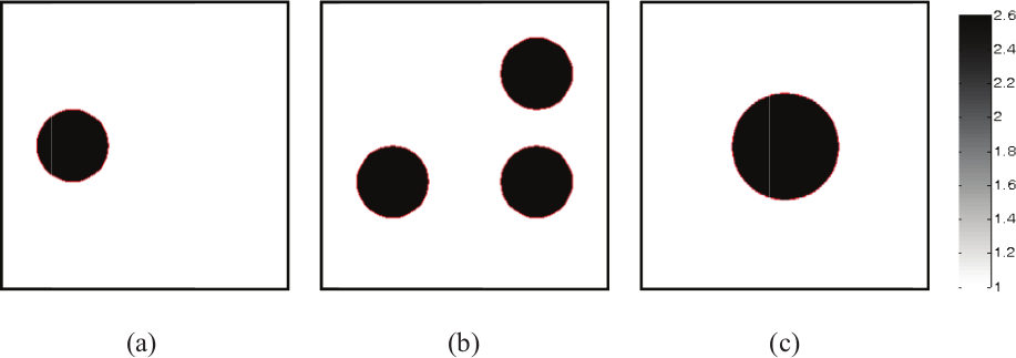
Original static reconstruction objects.
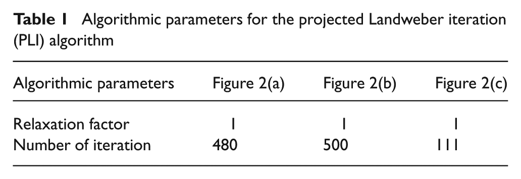
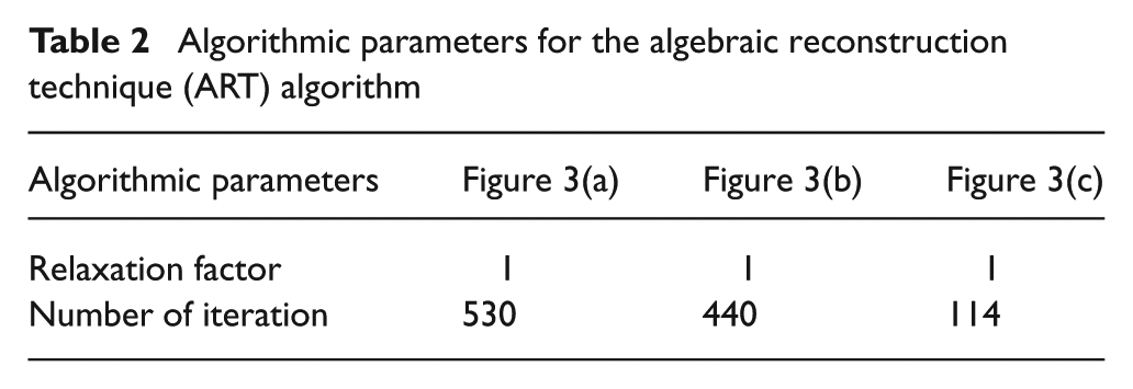
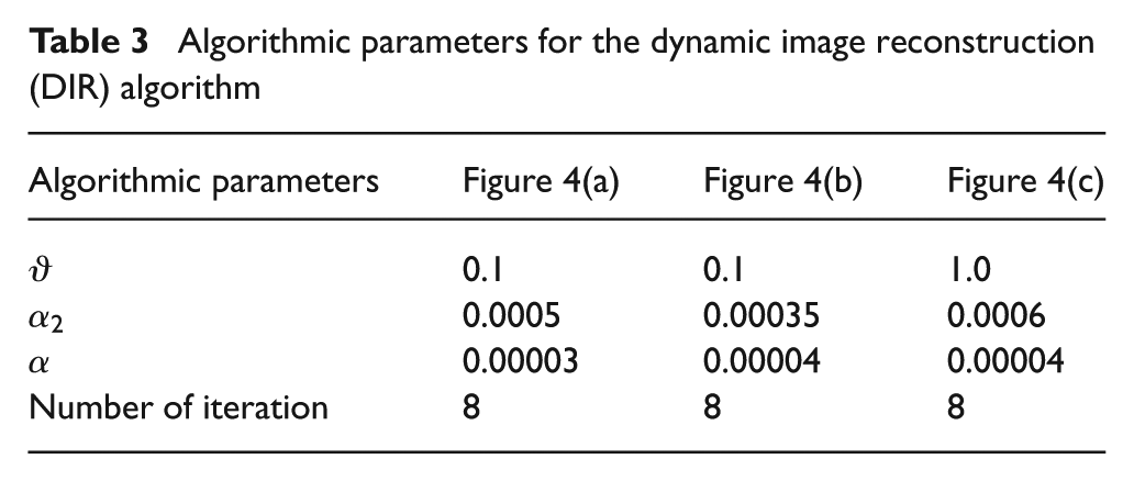
Tables 1 and 2 list the algorithmic parameters for the PLI algorithm and the ART algorithm, respectively. In the DIR algorithm,
Algorithmic parameters for the projected Landweber iteration (PLI) algorithm
Algorithmic parameters for the algebraic reconstruction technique (ART) algorithm
Algorithmic parameters for the dynamic image reconstruction (DIR) algorithm
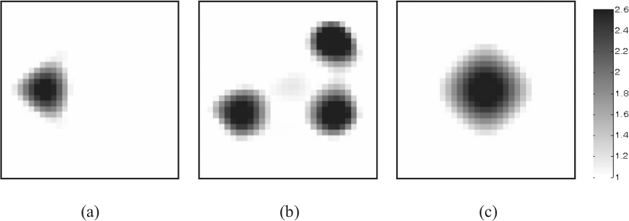
Reconstructed images by the projected Landweber iteration (PLI) algorithm.
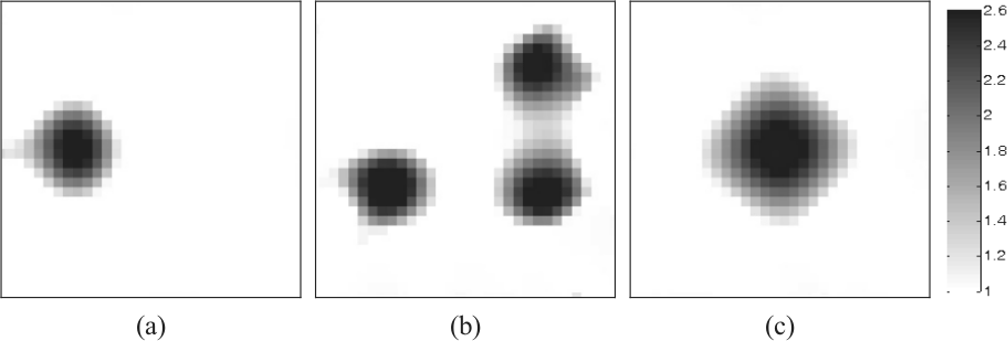
Reconstructed images by the algebraic reconstruction technique (ART) algorithm.
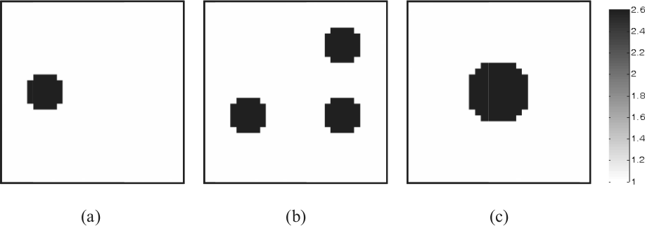
Reconstructed images by the dynamic image reconstruction (DIR) algorithm.
Image error (%)
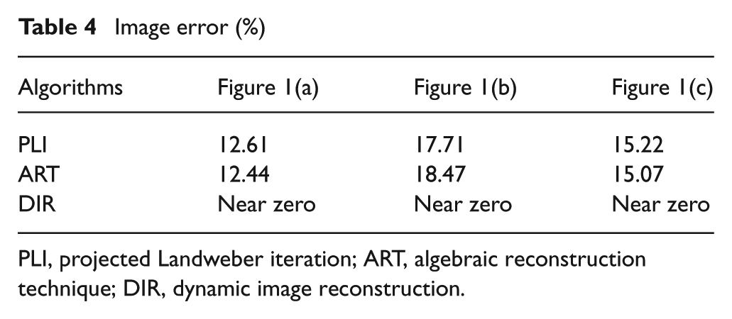
PLI, projected Landweber iteration; ART, algebraic reconstruction technique; DIR, dynamic image reconstruction.
Figure 2 shows the images reconstructed by the PLI algorithm. Numerical simulation results indicate that one of the distinct advantages of the PLI algorithm is that the numerical implementation is simple, and the computational complexity and cost are relatively low. For the cases simulated in this paper, unfortunately, the quality of the images reconstructed by the PLI method is far from perfect and the distortions are relatively serious, which indicate that it is difficult for the PLI algorithm to reconstruct the original objects exactly.
The images reconstructed by the ART algorithm are illustrated in Figure 3. Similarly, numerical simulation results reveal that the implementation of the ART algorithm is relatively easy, and the computational complexity and cost are low. However, it can be found from Figure 3 that for the cases simulated in this section, the quality of the images reconstructed by the ART algorithm is not satisfactory and the distortions of the reconstructed images are relatively large, which indicates that it is difficult for the ART algorithm to reconstruct detailed information on the original objects.
Figure 4 shows the images reconstructed by the DIR algorithm. Numerical simulation results indicate that the DIR algorithm shows a satisfactory numerical performance and can ensure the numerical stability of the solution owing to the fact that the Tikhonov regularization technique is used to stabilize the numerical solution. It can be seen from Figure 4 that the quality of the images reconstructed by the DIR algorithm is improved compared with the PLI algorithm and the ART method, the artifacts in the reconstructed images can be effectively eliminated and the distortion of the reconstructed images is very slight, which indicates that the DIR algorithm is successful in solving ECT inverse problems.
The image errors are listed in Table 4. The second and third rows in Table 4 are the image errors for the PLI algorithm and the ART algorithm. It can be observed that the quality of the images reconstructed by the PLI algorithm and the ART algorithm is not satisfactory and the distortions are relatively large. The fourth row in Table 4 shows the image errors for the DIR algorithm. As can be expected, the quality of the images reconstructed by the DIR algorithm is higher than the PLI method and the ART algorithm. For the cases simulated in this section, the DIR algorithm gives the smallest image errors, which indicates that the DIR algorithm is a promising candidate for solving ECT image reconstruction problems.
The CPU times for reconstructing subfigures a, b and c in Figure 2 using the PLI algorithm are about 0.68, 0.71 and 0.18 s. The CPU times for reconstructing subfigures a, b and c in Figure 3 using the ART algorithm are about 6.86, 5.71 and 1.48 s. The CPU times for reconstructing subfigures a, b and c in Figure 4 using the DIR algorithm are about 3.28 s. It can be found that for the cases simulated in this section, the reconstruction speed of the PLI algorithm is faster than the ART method and the DIR algorithm; however, the quality of the image reconstructed by the DIR algorithm is higher than the PLI method and the ART algorithm. In the future, more investigations on accelerating the DIR algorithm should be further implemented.
Case 2
Studies indicate that the ECT image reconstruction process is a typically ill-posed problem, and a small perturbation in the input data may bring a large fluctuation in the final results, which may make the inversion solution meaningless. Applications reveal that the noises in the capacitance measurement data are inevitable and complicated. A successful algorithm should have the advantage of dealing with the inaccurate properties on the capacitance measurement data. In this section, the noise-contaminated capacitance data are used to evaluate the numerical performance and robustness of the DIR algorithm, and the definition of the noise level can be found in Yang and Peng (2003). Algorithmic parameters for the DIR algorithm are the same as Table 3. Figures 5–7 illustrate the images reconstructed by the DIR algorithm under the noise levels of 1%, 6% and 15%. The image errors under different noise levels for the DIR algorithm are listed in Table 5.
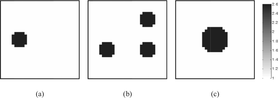
Reconstructed images by the dynamic image reconstruction (DIR) algorithm under the 1% noise level.
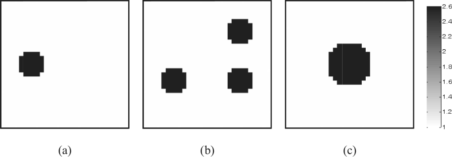
Reconstructed images by the dynamic image reconstruction (DIR) algorithm under the 6% noise level.
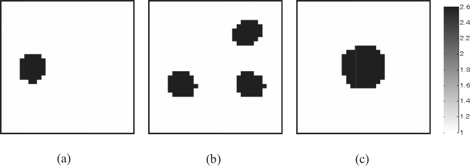
Reconstructed images by the dynamic image reconstruction (DIR) algorithm under the 15% noise level.
Image errors for the dynamic image reconstruction (DIR) algorithm under different noise levels (%)
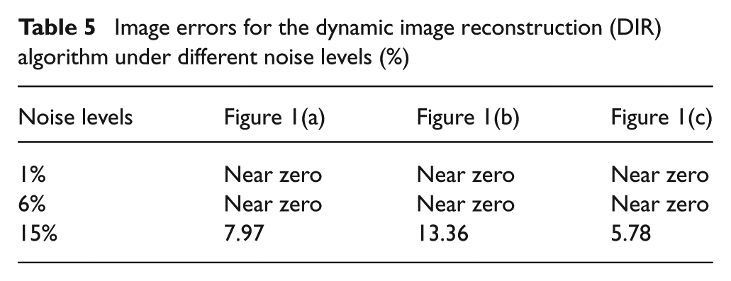
Figures 5–7 present the images reconstructed by the DIR algorithm under the noise levels of 1%, 6% and 15%. As can be expected, the DIR algorithm shows satisfactory numerical performance and the favourable robustness, and the artifacts in the reconstructed images can be effectively removed, which indicates that the DIR algorithm is successful in treating with the inaccuracies on the measurement data. Meanwhile, it can be observed from Table 5 that the quality of the images reconstructed by the DIR algorithm is acceptable under the noise levels simulated in the section. In particular, when the noise level is 15%, the image errors for the original reconstruction objects Figures 1(a–c) are 7.97%, 13.36% and 5.78%, which indicates that the DIR algorithm is robust. Additionally, it can be seen from Figures 5–7 and Table 5 that the quality of the reconstructed images decreases with the augmentation of the noise levels, which indicates that the inaccurate properties on the capacitance measurement data should be treated seriously, and this issue should be further investigated in the future.
Case 3
Applications indicate that ECT reconstruction objects are often in a dynamic process; a successful algorithm should be able to treat with such reconstruction tasks. In order to evaluate further the feasibility and efficiency of the DIR algorithm, a complicated dynamic reconstruction case, where the shapes and locations of the permittivity distributions change with the index of time, is simulated in this section. Subfigures (a), (b) and (c) in Figure 8 show the different permittivity distributions at discrete time indexes
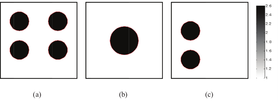
Original dynamic reconstruction objects.
The specific procedures on simulating the dynamic image reconstruction process can be summarized as: (1) the capacitance data (such as
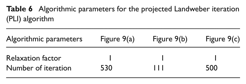
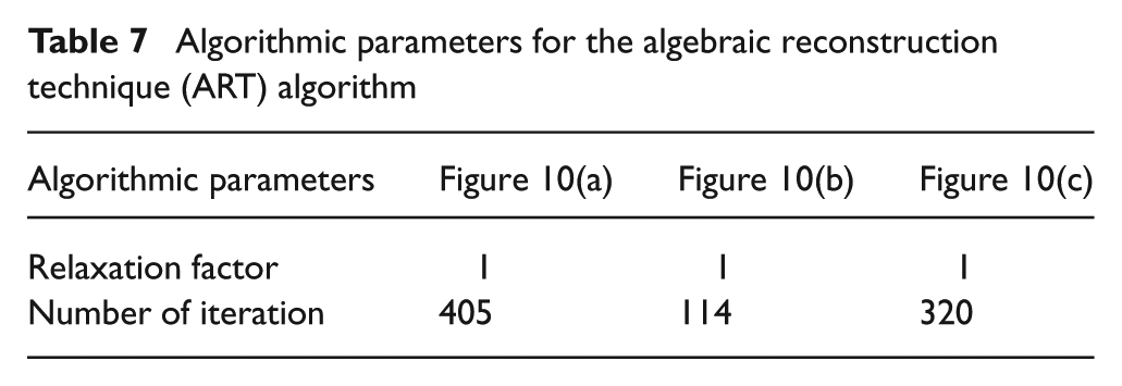
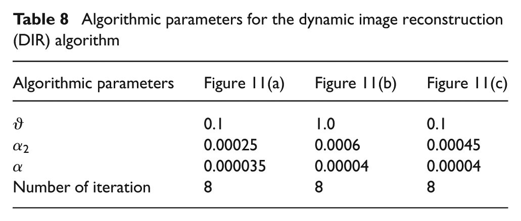
Tables 6 and 7 list the algorithmic parameters for the PLI algorithm and the ART method. Table 8 shows the algorithmic parameters for the DIR algorithm and the rest of the algorithmic parameters are the same as previously given. The images reconstructed by the PLI algorithm, the ART method and the DIR algorithm are illustrated in Figures 9–11. The image errors for the compared algorithms are presented in Table 9.
Algorithmic parameters for the projected Landweber iteration (PLI) algorithm
Algorithmic parameters for the algebraic reconstruction technique (ART) algorithm
Algorithmic parameters for the dynamic image reconstruction (DIR) algorithm
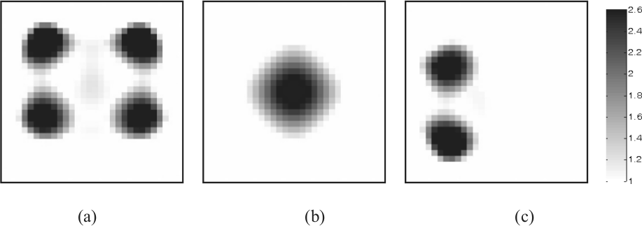
Reconstructed image by the projected Landweber iteration (PLI) algorithm.
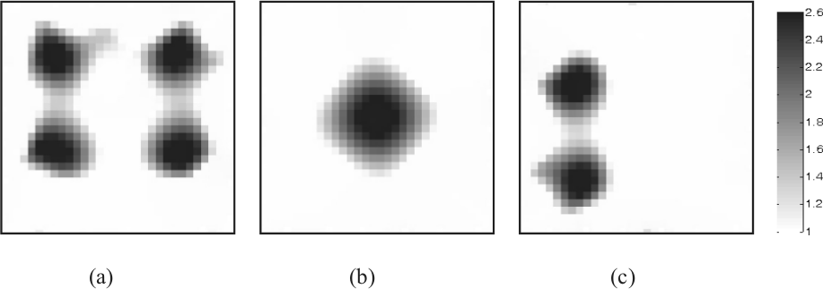
Reconstructed images by the algebraic reconstruction technique (ART) algorithm.
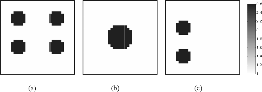
Reconstructed images by the dynamic image reconstruction (DIR) algorithm.
Image error (%)
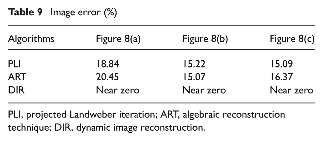
PLI, projected Landweber iteration; ART, algebraic reconstruction technique; DIR, dynamic image reconstruction.
Figures 9 and 10 present the images reconstructed by the PLI algorithm and the ART method under different time indexes. It can be observed that the distinct advantages of the PLI algorithm and the ART method include the easy implementation, the low computational complexity and cost. For the dynamic reconstruction cases simulated in the section, however, the quality of the images reconstructed by the PLI algorithm and the ART method is far from satisfactory and the distortions are relatively serious. Additionally, it is worth mentioning that ECT reconstruction objects are often in a complicated dynamic evolution process; the PLI algorithm and the ART method merely consider the ECT measurement information and fail to consider the dynamic evolution information of the objects of interest. As a result, it is hard for the PLI algorithm and the ART method to reconstruct the complicated dynamic objects exactly.
The images reconstructed by the DIR algorithm under different time indexes are shown in Figure 11. As can be expected, when the dynamic reconstruction objects are considered, the DIR algorithm shows satisfactory numerical performance, the quality of the images reconstructed by the DIR algorithm is improved compared with the PLI algorithm and the ART method, and the artifacts in the reconstructed images can be effectively eliminated. In addition, it can be found from Figures 9–11 that the quality of the images reconstructed by the DIR algorithm is higher than the PLI algorithm and the ART method, which indicates that the DIR algorithm is successful in solving ECT inverse problems.
Table 9 lists the image errors for the PLI algorithm, the ART method and the DIR algorithm. It can be observed from Table 9 that for the dynamic reconstruction objects, the quality of the images reconstructed by the PLI algorithm and the ART method is not satisfactory and the image errors are relatively large. It can be seen from Table 9 that for the dynamic reconstruction cases simulated in this section, the DIR algorithm gives the smallest image errors, which indicates that the DIR algorithm is successful in solving ECT image reconstruction problems.
Case 4
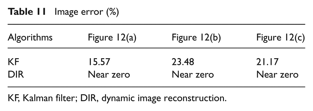
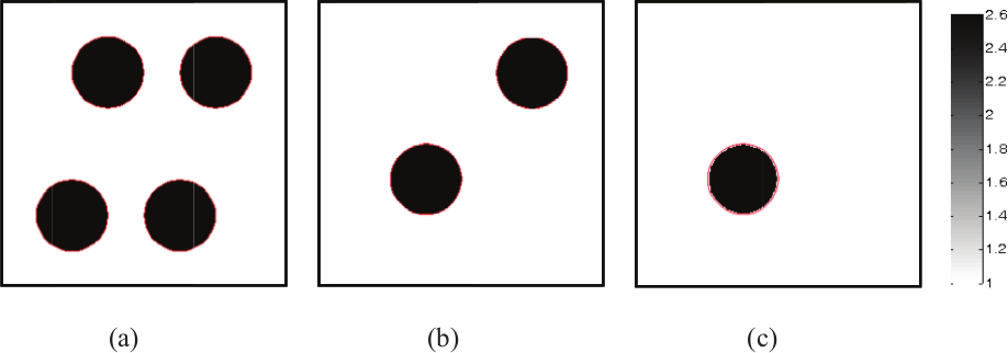
In order to evaluate further the feasibility and effectiveness of the DIR algorithm, another dynamic reconstruction case is simulated in this section. Especially, the quality of the images reconstructed by the DIR algorithm is compared with the KF method (one of the typical dynamic reconstruction algorithms). Subfigures (a), (b) and (c) in Figure 12 represents the different locations of the dynamic reconstruction objects at discrete time indexes
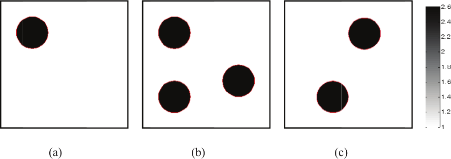
Original dynamic reconstruction objects.
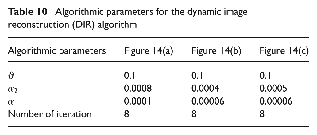
Algorithmic parameters for the dynamic image reconstruction (DIR) algorithm
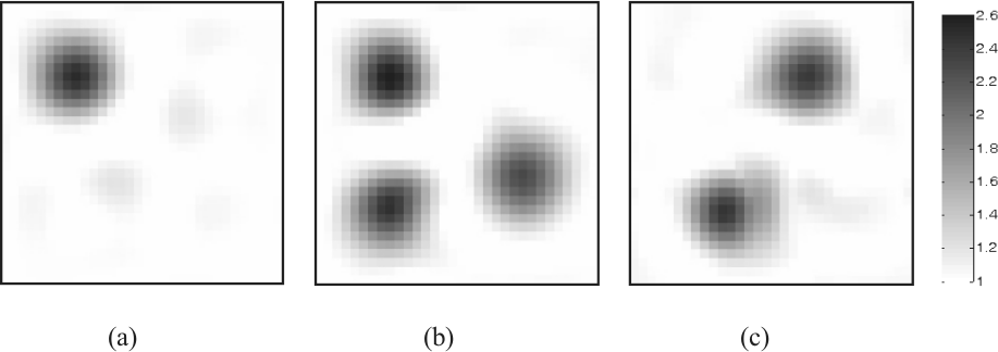
Reconstructed image by the Kalman filter (KF) method.
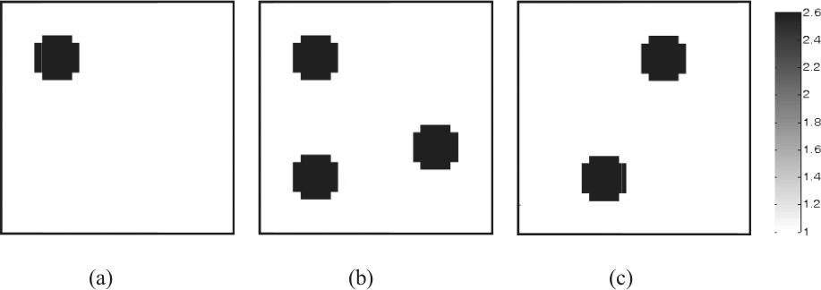
Reconstructed images by the dynamic image reconstruction (DIR) algorithm.
Image error (%)
KF, Kalman filter; DIR, dynamic image reconstruction.
The images reconstructed by the KF method under different time indexes are illustrated in Figure 13. It can be observed that the distinct advantages of the KF method include the easy numerical implementation and the low computational complexity and cost. For the dynamic reconstruction cases simulated in the section, however, the quality of the images reconstructed by the KF method is far from satisfactory, the distortions are relatively serious and the artifacts are comparatively more. In addition, the results in Figure 13 indicate that it is hard for the KF method to reconstruct the original dynamic objects exactly.
The images reconstructed by the DIR algorithm under different time indexes are presented in Figure 14. As can be expected, when the dynamic reconstruction objects are considered, the DIR algorithm shows satisfactory numerical performance, the quality of the images reconstructed by the DIR algorithm is improved compared with the KF method, and the artifacts in the reconstructed images can be eliminated effectively. Meanwhile, it can be observed from Figures 13 and 14 that the quality of the images reconstructed by the DIR algorithm is higher than the KF method, which confirms that the DIR algorithm is successful in imaging the dynamic objects.
Table 11 lists the image errors for the KF method and the DIR algorithm. The second row in Table 11 is the image errors for the KF method. It can be observed that for the dynamic reconstruction objects, the quality of the images reconstructed by the KF method is far from perfect. The third row in Table 11 lists the image errors for the DIR algorithm. As can be expected, in the cases of the dynamic reconstruction objects, the quality of the images reconstructed by the DIR algorithm is higher than the KF method. Meanwhile, it can be observed from Table 11 that for the dynamic reconstruction cases simulated in this section, the DIR algorithm gives the smallest image errors, which indicates that the DIR algorithm is a promising candidate for solving the dynamic reconstruction problems.
Case 5
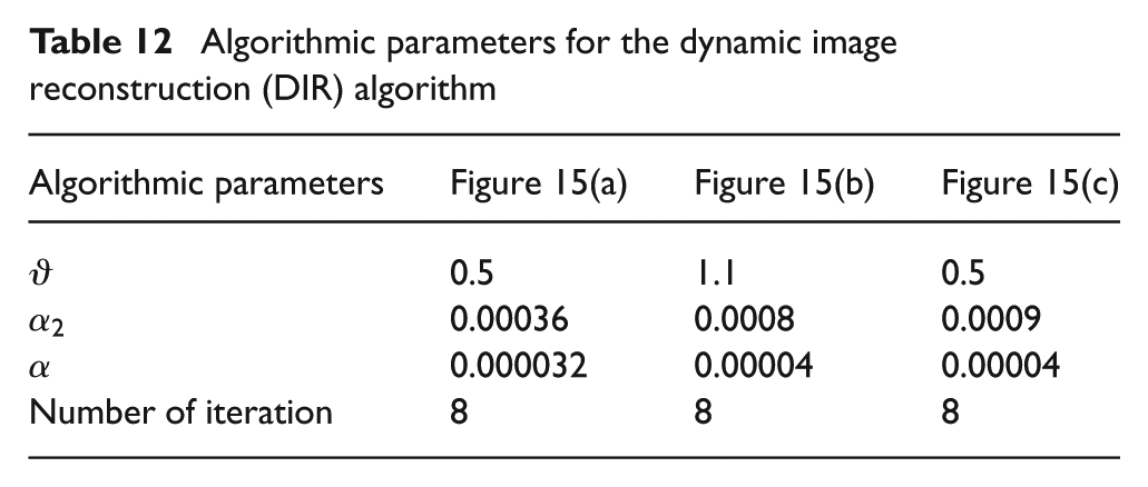
In this section, to evaluate further the feasibility and robustness of the DIR algorithm, another dynamic reconstruction case is simulated. In order to simulate real measurement environment, the noise-contaminated capacitance data is used. Figure 15 shows the dynamic process of the objects of interest under different time indexes, and subfigures a, b and c in Figure 15 represents the different locations of the dynamic reconstruction objects at discrete time indexes
Original dynamic reconstruction objects.
Algorithmic parameters for the dynamic image reconstruction (DIR) algorithm
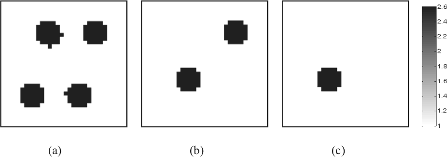
Reconstructed images by the dynamic image reconstruction (DIR) algorithm under the 5% noise level.
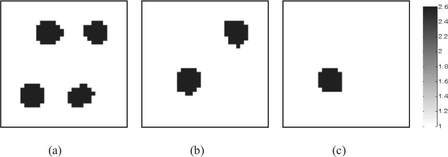
Reconstructed images by the dynamic image reconstruction (DIR) algorithm under the 13% noise level.
Image error (%)
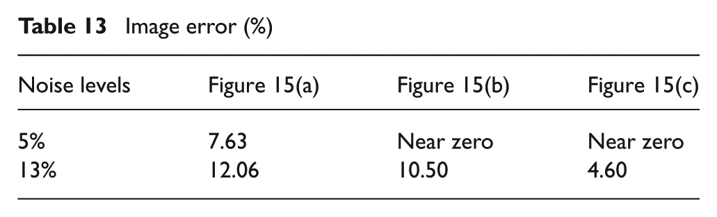
Figures 16 and 17 illustrate the images reconstructed by the GIR algorithm under the noise levels of 5% and 13%. As can be expected, when the measurement noises in the dynamic reconstruction objects are considered, the DIR algorithm shows satisfactory robustness and the quality of the images reconstructed by the DIR algorithm is acceptable. It can be seen from Figures 16 and 17 and Table 13 that the quality of the reconstructed images decreases with the increase of the noise levels, which indicates that the inaccurate properties on the measurement data should be treated seriously, and the issue should be further investigated in the future.
Conclusions
ECT is considered a promising visualization measurement technology, in which reconstructing high-quality images is highly desirable for real applications. Applications indicate that ECT measurement objects are often in a complicated dynamic process, and developing a dynamic reconstruction algorithm to image a dynamic object is important for real applications. In this paper, a dynamic reconstruction model, which integrates the ECT measurement information and the dynamic evolution information of the reconstruction objects, is presented. A generalized objective function, which simultaneously considers the ECT measurement information, the dynamic evolution information of the dynamic objects of interest, the temporal constraints and the spatial constraints, is proposed. An iteration scheme that integrates the advantages of the split Bregman iteration technique and the homotopy method is developed for solving the proposed objective function. Numerical simulations are implemented to evaluate the feasibility and effectiveness of the proposed algorithm. For the cases simulated in this paper, the accuracy of the images reconstructed by the proposed algorithm is improved and the artifacts in the reconstructed images can be removed effectively, which indicates that the proposed algorithm is successful in solving ECT inverse problems. As a result, a promising algorithm is introduced for solving ECT image reconstruction problems.
Applications indicate that each algorithm may illustrate different numerical performances to different reconstruction tasks, and the selection of a specific image reconstruction algorithm depends mainly on the measurement requirements and the prior information of a specific reconstruction task. Our work provides an alternative approach for solving ECT inverse problems, which needs to be further validated by more cases in the future.
Footnotes
Funding
This work was supported by the Fundamental Research Funds for the Central Universities (No. 10MG20); the China Postdoctoral Science Foundation (Nos. 20090460263 and 201003088); the National Natural Science Foundation of China (Nos. 50736002, 51006106 and 50906086); and the Program for the Changjiang Scholars and Innovative Research Team in University (No. IRT0952).