






Abstract
The image reconstruction task in electrical capacitance tomography (ECT) is an ill-posed problem, in which image reconstruction methods play a vital role in real applications. In this paper, a multiple measurement vector-based dimensionality reduction dynamic reconstruction model that simultaneously utilizes the ECT measurement information and the dynamic evolution information of a dynamic object is proposed. A robust sparse orthogonal projective non-negative matrix factorization (RSOPNMF) method is proposed for extracting the basis vectors from a set of snapshots, and the split Bregman iteration (SBI) algorithm is used to solve the RSOPNMF model. The original unknown variables are projected onto the subspaces spanned by a set of the basis vectors extracted by the RSOPNMF method from a set of snapshots to obtain a low-dimensional model, where the images are indirectly reconstructed by solving the corresponding low-dimensional coefficient vector, and thus the dimensionality of the unknown variables is reduced and the computational cost are decreased. Based on the multiple measurement vectors and the dimensionality reduction model, an objective functional that incorporates the ECT measurement information, the dynamic evolution information of a dynamic object, the spatial constraint and the temporal constraint is proposed, in which the unknown variables are solved in a batching pattern. An iterative scheme that integrates the beneficial advantages of the SBI method and the forward–backward splitting algorithm is developed for solving the proposed objective functional. Numerical simulation results validate the feasibility of the proposed algorithm.
Keywords
Introduction
The electrical capacitance tomography (ECT) measurement method attempts to acquire the permittivity distribution information of the cross-section from the given capacitance measurement data via an appropriate algorithm, in which reconstruction algorithms play a crucial role in real applications. The ECT image reconstruction task consists of two major procedures: the forward problem and the inverse problem. The former is a well-posed problem with a purpose of computing the capacitance values from the given permittivity distributions, which can be easily solved by different numerical methods such as the finite element method and the finite difference method. According to the inverse problem theory (Engl et al., 2000; Han and Li, 2011; Huang and Zhao, 2005; Kirsch, 1996; Liu, 2005; Tarantola, 2005; Tikhonov and Arsenin, 1977; Vogel, 2002; Wang, 2007), the latter is an ill-posed problem with a motivation of estimating the permittivity distributions from the finite capacitance data.
In a mathematical notation, the relationship between the capacitance and the permittivity distribution is governed by (Yang and Peng, 2003):
where
where
Reconstructing high-quality images is desired for real applications. In the past few years, various algorithms, including static reconstruction algorithms and dynamic reconstruction methods, have been developed for ECT image reconstruction. Common static reconstruction algorithms include the linear back-projection algorithm (Xie et al., 1992), the standard Tikhonov regularization (STR) method (Tikhonov and Arsenin, 1977), the Landweber iteration technique (Jang et al., 2006; Landweber, 1951; Yang et al., 1999), the neural network algorithm (Warsito and Fan, 2001), the truncated singular value decomposition method (Yang and Peng, 2003), the algebraic reconstruction technique (ART; Yang and Peng, 2003), the simultaneous iterative reconstruction technique (SIRT; Yang and Peng, 2003), the offline iteration and online reconstruction technique (Liu et al., 2004), the generalized Tikhonov regularization algorithms (Fang, 2004; Soleimani and Lionheart, 2005; Wang et al., 2007), the simulated annealing method (Ortiz-Aleman et al., 2004), the genetic algorithm (Mou et al., 2005), the generalized vector sampled pattern matching (GVSPM) method (Takei, 2006), the non-linear Landweber iteration algorithm (Li and Yang, 2008), the level set method (Banasiak and Soleimani, 2010; Kortschak et al., 2007), the Calderon method (Cao et al., 2011) and the image fusion-based method (Olmos et al., 2012). Popular dynamic reconstruction algorithms include the particle filter algorithm (Watzenig et al., 2007), the Kalman filter method (Soleimani et al., 2007), the four-dimensional imaging technique (Soleimani et al., 2009), the Ensemble Kalman filter method (Lei et al., 2012) and the split Bregman iteration (SBI)-based reconstruction algorithm (Lei et al., 2013); more details on the filter-based methods can be found in Zhu (2010). In the past few years, static reconstruction methods have been intensively studied. Owing to the fact that the considerations of the dynamic evolution information of a dynamic object and the temporal correlations are absent, however, static reconstruction methods may not be optimal for dynamic remonstration tasks. Due to the complexities and particularities of the dynamic reconstruction tasks, currently the investigations on dynamic reconstruction algorithms are far from perfect, and seeking an efficient reconstruction method that achieves fast and high-quality reconstruction remains a critical issue.
In order to address the above challenges, naturally, the main motivation of the paper is to improve the reconstruction speed and the reconstruction quality, and the main contributions are outlined as follows.
A dimensionality reduction-based multiple measurement vectors dynamic reconstruction model that utilizes the ECT measurement information and the dynamic evolution information of a dynamic object is proposed.
A robust sparse orthogonal projective non-negative matrix factorization (RSOPNMF) method is proposed for extracting the basis vectors from a set of snapshots, the original unknown variables are projected onto the subspaces spanned by the set of the basis vectors to obtain a low-dimensional model where the images are indirectly reconstructed by solving a low-dimensional RSOPNMF coefficient vector, and thus the dimensionality of the unknown variables is reduced, the underdetermined property is alleviated, the computational cost is decreased and the reconstruction speed is improved.
Based on the multiple measurement vectors and the dimensionality reduction model, a new objective functional that integrates the dynamic evolution information of the objects of interest, the ECT measurement information, the temporal constraint and the spatial constraint is proposed, in which the images are reconstructed by a batching pattern.
An iteration scheme that integrates the beneficial advantages of the SBI method and the forward–backward splitting (FBS) algorithm is developed for solving the proposed objective functional. Numerical simulations are implemented to validate the feasibility of the proposed algorithm. More importantly, this paper proposes a general framework for ECT image reconstruction problem, which may be applicable for other related tomography problems.
The rest of this paper is structured as follows. In the next section, a RSOPNMF method is proposed, then an iterative scheme is proposed for solving the RSOPNMF model, and finally a RSOPNMF-based dimensionality reduction model is proposed. A multiple measurement vector-based dimensionality reduction dynamic reconstruction model is presented, and an objective functional that fuses the dynamic evolution information of a dynamic object, the ECT measurement information, the temporal constraint and the spatial constraint is proposed. An iteration scheme, which integrates the merits of the SBI method and the FBS algorithm, is developed for solving the proposed objective functional. Numerical simulation results and discussions are illustrated and finally, conclusions are presented.
RSOPNMF-based dimensionality reduction method
In common reconstruction algorithms, including static and dynamic reconstruction algorithms, the original unknown variables are directly reconstructed, which is therefore not appropriate for imaging a dynamic object because of the time-consuming computation process. In this section, the non-negative matrix factorization (NMF) approach and the projective non-negative matrix factorization (PNMF) method are concisely introduced, a new RSOPNMF method is proposed for extracting the basis vectors from a set of snapshots, and the SBI method is developed for solving the RSOPNMF model. Finally, a procedure of extracting the basis vectors from the set of snapshots is outlined and a RSOPNMF-based dimensionality reduction method is presented.
Non-negative matrix factorization
The principle component analysis (PCA) method is an effective data processing approach. One of the important characteristics in the PCA method is that data representation is not purely additive, i.e. each principle component consists of both negative and positive entries. The linear combination in the PCA subspace mixes with both positive and negative weights, which are likely to cancel each other partially in the data representation. Finally, the partial cancellations lead to the loss of data in the PCA method (Han, 2010). Additionally, the negative components in the PCA method are hard to explain for specific applications, such as an ECT image.
The NMF method attempts to recover the hidden non-negative structures or patterns from the redundant data. Differing from common PCA method, the NMF method is a parts-based representation of an ensemble of signals or images. Far beyond a mathematical exploration, the philosophy underlying the NMF method, which tries to formulate a feasible model for learning object parts, is closely relevant to the perception mechanism. While the parts-based representation seems intuitive, it is indeed on the basis of physiological and psychological evidence: perception of the whole is based on the perception of its parts (Choi, 2008; Cichocki et al., 2009; Ding et al., 2006; Lee and Seung, 1999, 2001; Wang and Zhang, 2013). In fact, there are two complementary connotations in non-negativity (or non-negative component) and purely additive combination. On the one hand, the negative values of both observations and the latent components are physically meaningless in numerous real applications, such as an ECT image. On the other hand, objects of interest are most naturally characterized by the inventory of its parts, and the exclusively additive combination means that they can be reassembled by adding required parts together similar to identikits (Choi, 2008; Cichocki et al., 2009; Ding et al., 2006; Lee and Seung, 1999, 2001; Wang and Zhang, 2013).
Given an input data matrix
where
In order to obtain the non-negative decompositions of a non-negative matrix, the NMF problem is cast as an optimization problem (Cichocki et al., 2009):
RSOPNMF
The PNMF method is derived from the NMF technique, which is introduced to improve the locality of the part-based representations, and it can be formulated as (Yang et al., 2007; Yang and Oja, 2010):
where
In real ECT applications, data matrix
where
In practice, imposing additional orthogonality and sparsity constraints is useful. In particular, an orthogonal matrix will form a basis of a subspace, and thus it will facilitate the geometric interpretation and the data reconstruction. Finally, a RSOPNMF method with the orthogonality and sparsity constraints on
where
Proposed iterative scheme
Equation (7) involves two unknown matrix variables,
Finally, it can be observed from Equations (8) and (9) that the algorithmic structure can be expressed as an iterative series
According to the SBI method (Cai et al., 2009a, 2009b; Goldstein and Osher, 2009; Goldstein et al., 2010; Osher et al., 2010; Yin et al., 2008; Zhang et al., 2011b), Equation (10) is iteratively solved by:
For the sake of easy computation, similarly, Equation (11) can be decoupled as the following two sub-problems (Blondel et al., 2013; Chan and Wong, 2000; Lv et al., 2013; Qin et al., 2013; Tseng, 2001; Xiao et al., 2011; Xu and Yin, 2013):
Commonly, Equation (14) can be solved using the standard Lagrangian multipliers method by introducing the orthogonality constraint to the objective functional. For the sake of easy computation, however, applying the natural gradient on the Stiefel manifold to impose the orthogonality constraint on matrix
where
Based on the multiplicative update rule (Choi, 2008; Cichocki et al., 2009; Ding et al., 2006; Edelman et al., 1999; Lee and Seung, 2001; Nishimori and Akaho, 2005; Yoo and Choi, 2010) and Equation (14), finally, an iteration scheme of solving matrix variable
where
According to the above discussions, an iterative scheme is proposed for solving Equation (7), which can be summarized as follows:
Step 1. Specify the algorithmic parameters and the initial values.
Step 2. A set of snapshots is generated by measurement methods or numerical solutions or a combination of the two approaches.
Step 3. Update
Step 4. Update
Step 5. Update
Step 6. Update
Step 7. Loop to Step 3 until a predetermined stopping criterion is satisfied.
RSOPNMF-based dimensionality reduction method
Following the above discussions, if a basis matrix
where
According to the discussions presented in previous sections, finally, a RSOPNMF-based dimensionality reduction approach can be outlined as follows:
Step 1. A set of snapshots is generated.
Step 2. Extract the basis vectors from a set of snapshots using the proposed iterative scheme presented above.
Step 3. Use the basis vectors to represent an unknown matrix, and thus a low-dimensional model is obtained.
Reconstruction model
The common reconstruction model, Equation (2), considers the inaccuracy of the capacitance measurement data. Studies indicate that the model approximation deviations derived from the approximation and discretization of a real problem and physically implementing an ECT sensor will undoubtedly introduce errors, and thus developing a model that simultaneously considers the inaccurate properties on the capacitance measurement data, the model approximation and the sensitivity matrix may be essential for improving the reconstruction quality. Differing from vector-based reconstruction models, in this paper a multiple measurement vector-based reconstruction model considering the above inaccurate properties can be formulated as:
where
Commonly, the dynamic evolution process of a dynamic object in real applications can be generally depicted by the following formula:
where
ECT imaging objects are often in a fast dynamic process. To visualize the detailed characteristics of the dynamic process, achieving fast reconstruction is essential, and thus introducing the linearization approximation to Equation (19) yields:
where
Finally, a dynamic reconstruction model that integrates the ECT measurement information and the dynamic evolution information of a dynamic object is formulated as:
In common static and dynamic reconstruction methods, the number of the unknown variables is more than that of the independent equations, which restricts the improvement of the reconstruction speed. Differing from common reconstruction methods, in this paper the original unknown variables are projected onto the spaces spanned by the basis vectors extracted by the RSOPNMF method to reduce the dimensionality of the unknown variable, and a dimensionality reduction dynamic image reconstruction model can be formulated as:
Objective functional
In order to ensure a stable numerical solution, the Tikhonov regularization method is employed to solve Equation (22), and thus the equation can be cast as the following optimization problem:
where
To improve the robustness of the least squares estimation, in this paper the absolute value function is used to replace the squared residuals (Cichocki and Amari, 2002; Huber 1981), and thus Equation (23) is reformulated by:
where
For the sake of easy computation,
Finally, an objective functional for ECT reconstruction is specified as:
Equation (29) belongs to the framework of the Tikhonov regularization method, which has the following desirable properties:
Differing from common reconstruction algorithms, in which the unknown variables are directly reconstructed, the dimensionality of the unknown variables in Equation (29) is reduced by the RSOPNMF method, which will facilitate the improvement of the reconstruction speed.
The prior information from previous measurement or numerical simulations can be integrated to Equation (29) in solving the basis vectors, and thus the quantity of information is indirectly increased.
The dynamic evolution information of a dynamic object and the ECT measurement information are exploited in Equation (29), and thus the quantity of information in ECT image reconstruction is increased, and it will facilitate the improvement of the reconstruction quality.
Owing to the fact that it is hard to describe exactly the dynamic evolution information of the objects and to achieve exact capacitance measurements, the inaccurate properties of the dynamic evolution information and the measurement information are emphasized in Equation (29). In the measurement equation, particularly, the measurement noises, the model approximation deviations and the inaccuracy of the sensitivity matrix are simultaneously considered, which distinctly differs from common dynamic and static reconstruction algorithms.
The spatial constraint and the temporal constraint are simultaneously emphasized in Equation (29). In the case of the multiple measurement vectors, especially, the temporal constraint is introduced to impose the temporal correlations of a dynamic object.
The unknown variables in Equation (29) are three matrices, and it differs from other vector-based reconstruction algorithms, such as the ART method, the GVSPM algorithm, etc. In particular, the images are reconstructed by a batching pattern in Equation (29), which will facilitate the exploitation of the temporal correlations of a dynamic object and the improvement of the reconstruction speed.
Owing to the ill-posed nature of the inverse problem, ECT inversion solution is unstable, that is, a small fluctuation in the input data may bring a fatal effect on final results, which may make the inversion solution meaningless. As a result, methods that ensure a stable numerical solution while improving the reconstruction quality should be used. In Equation (29), the Tikhonov regularization technique is introduced to stabilize an inversion solution.
In real applications, measurement noises are ubiquitous and complicated. In Equation (29), the robust estimation is employed to improve the robustness of estimation.
Solving of the objective functional
Seeking an efficient algorithm to solve Equation (29) is crucial. In this section, the FBS algorithm is introduced, and an iteration scheme that integrates the merits of the SBI method and the FBS algorithm is proposed for solving Equation (29).
Forward–backward splitting method
Owing to the low computational complexity, the FBS algorithm is used to solve the proposed objective functional. In a mathematical notation, the FBS method aims at solving the following optimization problem (Combettes and Wajs, 2005; Duchi and Singer, 2009; Montefusco et al., 2011; Zhang et al., 2010):
where
After the corresponding deductions, the final FBS algorithm is formulated as:
where the proximal operator
In the case of
Proposed iteration scheme
According to the optimization theory, Equation (29) is reformulated as a constrained optimization problem by introducing an equality constraint:
Applying the SBI algorithm to Equation (35) yields:
There are four unknown variables in Equation (36), and efficiently solving the equation is crucial. For the sake of easy computation, following the computational strategies presented in Blondel et al. (2013), Chan and Wong (2000), Lv et al. (2013), Qin et al. (2013), Tseng (2001), Xiao et al. (2011) and Xu and Yin (2013), it is numerically appealing to decouple Equation (36) as:
Following the discussions presented in previous sections, an iteration scheme is proposed for solving Equation (29), which is outlined as follows:
Step 1. Specify the algorithmic parameters and the initial values.
Step 2. Obtain
Step 3. Update variable
Step 4. Update variable
Step 5. Update variable
Step 6. Update variable
Step 7. Update variable
Step 8. Loop to Step 3 until a predetermined iteration stopping criterion is satisfied.
Step 9. Solve Equation (17) to obtain the estimation of the original unknown variable.
Numerical simulations and discussions
For simplicity, the proposed method is called as the RSOPNMF-based dynamic reconstruction (RSOPNMFDR) algorithm. In this section, the dynamic reconstruction cases with multiple measurement vectors are implemented to numerically evaluate the feasibility and effectiveness of the RSOPNMFDR algorithm, and the reconstruction quality and speed are compared with the projected Landweber iteration (PLI) method. The robustness of the RSOPNMFDR algorithm is evaluated using the noise-contaminated capacitance data. Additionally, the effect of the number of the basis vectors on the reconstruction quality is numerically exploited.
A 12-electrode square ECT sensor is selected for simulations and an image is visualized using 32×32 pixels. All algorithms are implemented using the MATLAB 7.0 software on a PC with a Pentium IV 2.4-GHz CPU and 4 Gbytes memory. In this paper, the image error is used to evaluate the quality of an inversion solution, which can be specified as:
where
Case 1
In this section, numerical simulations are implemented to evaluate the feasibility and effectiveness of the RSOPNMF method, and the initial value is solved by the singular values decomposition method. Figure 1 illustrates the basis vectors extracted by the RSOPNMF method from a set of snapshots and Figure 2 shows the orthogonality of the basis matrix.
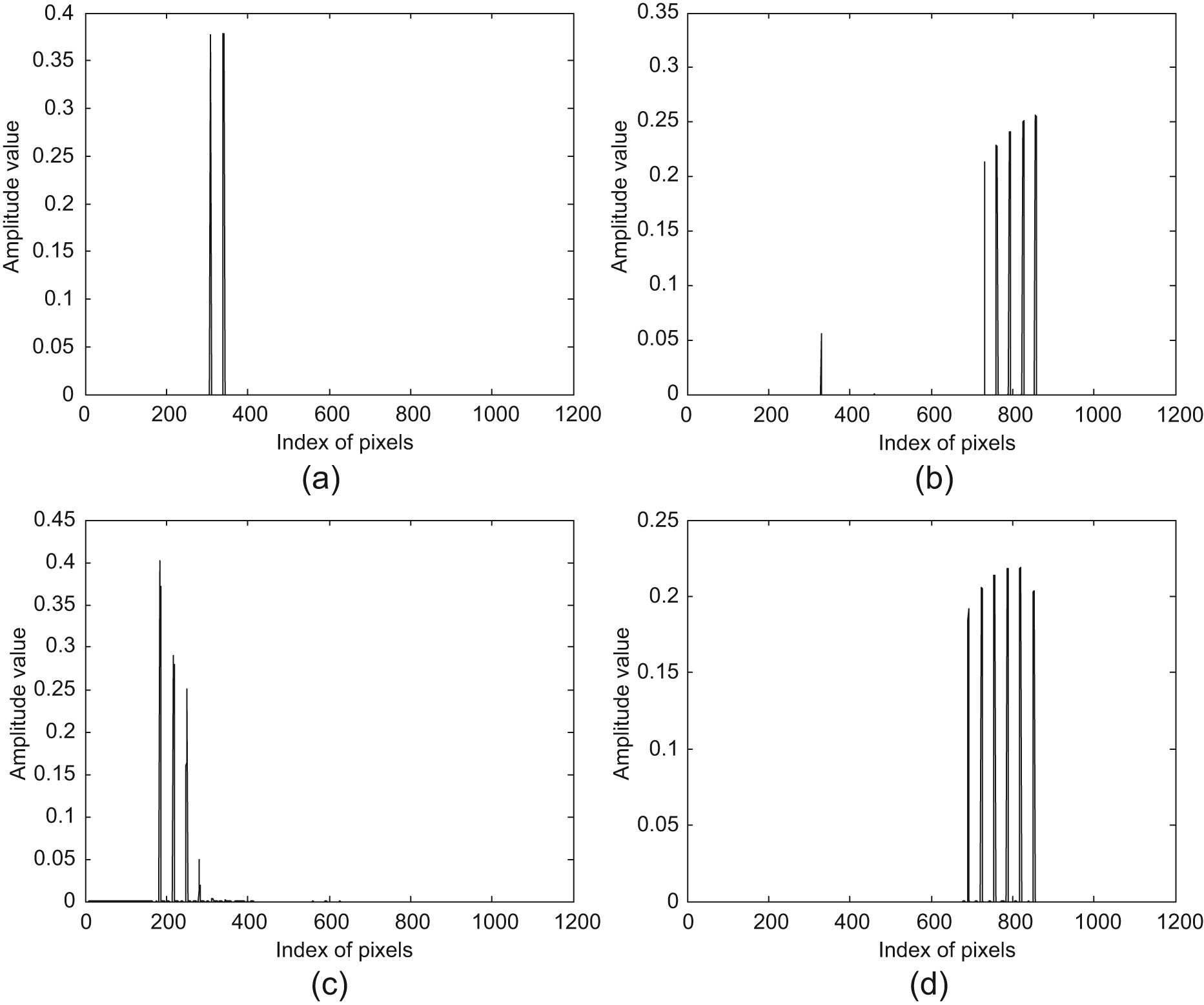
Basis vectors: (a) the third basis vector; (b) the 10th basis vector; (c) the 16th basis vector; (d) the 23rd basis vector.
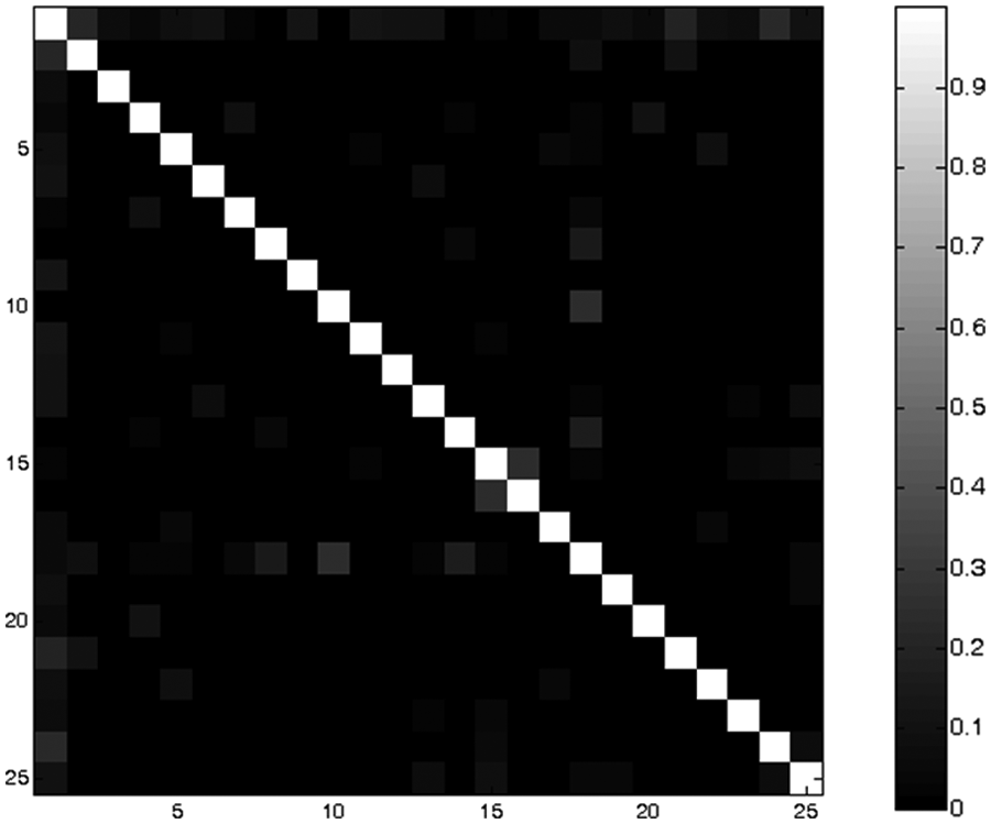
Orthogonality of the basis matrix.
Four basis vectors extracted by the RSOPNMF method are shown in Figure 1. It can be found from Figure 1 that differing from the common PCA method, the RSOPNMF method can ensure the sparseness and non-negativity of a basis vector, which indicates that the RSOPNMF algorithm is successful in exacting the basis vectors. It is worth emphasizing that the basis vectors can be in advance solved, which will not influence the reconstruction speed.
In practice, the orthogonality of the basis matrix is highly useful. In particular, an orthogonal matrix will form a basis of a subspace, and thus facilitates the geometric interpretation and the data reconstruction. Figure 2 illustrates the orthogonality of the basis matrix, that is, the image of the matrix
Case 2
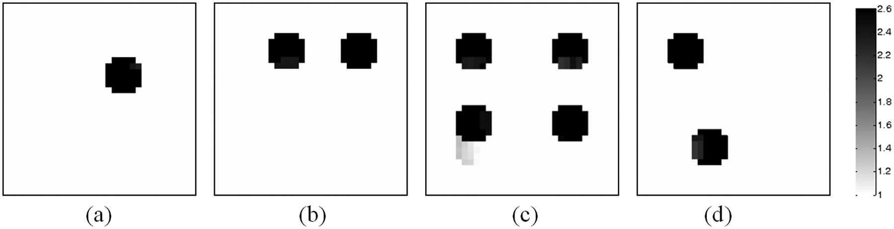
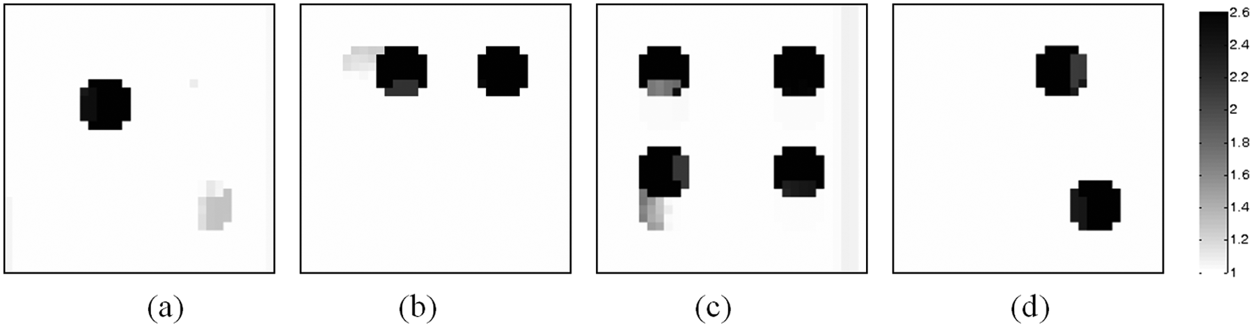
ECT imaging objects are often in a dynamic process, a successful algorithm should be able to tackle such reconstruction tasks. In this section, a dynamic reconstruction case is simulated to evaluate the feasibility of the RSOPNMFDR algorithm. Subfigures (a), (b), (c) and (d) in Figure 3 stand for the different permittivity distributions at time instants
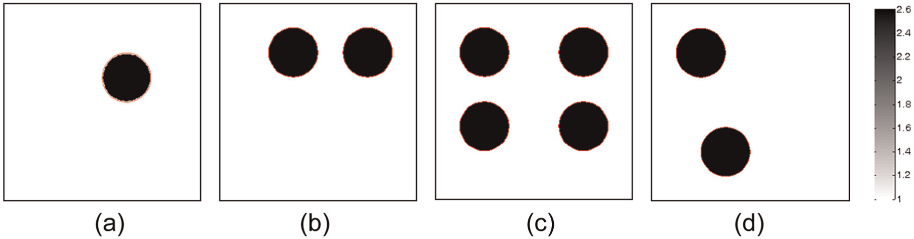
Reconstruction objects.
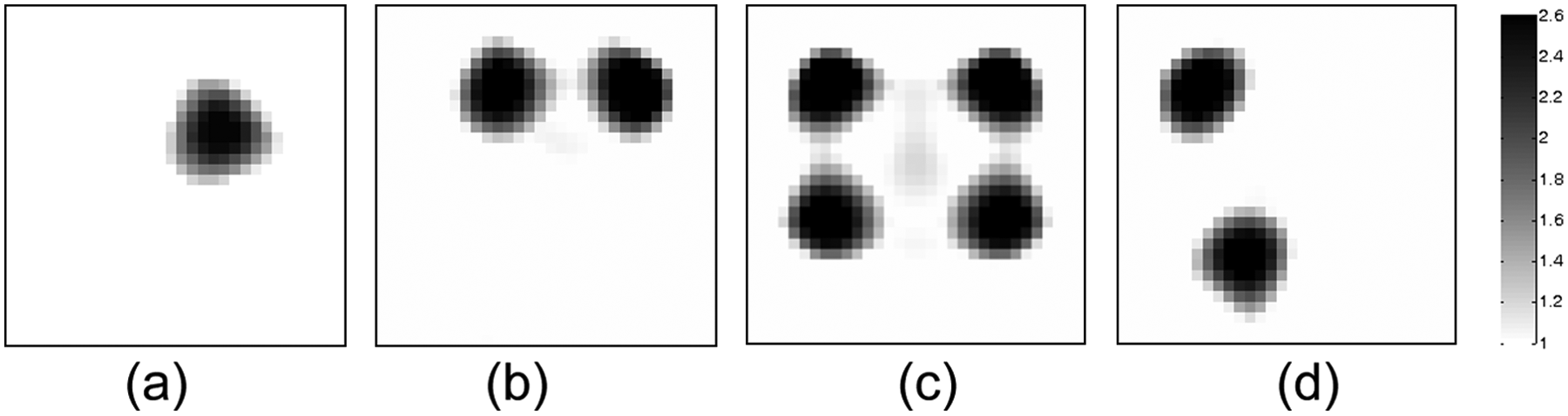
Reconstructed images by the projected Landweber iteration (PLI) algorithm.
Reconstructed images by the robust sparse orthogonal projective non-negative matrix factorization-based dynamic reconstruction (RSOPNMFDR) algorithm.
Algorithmic parameters for the projected Landweber iteration (PLI) algorithm.
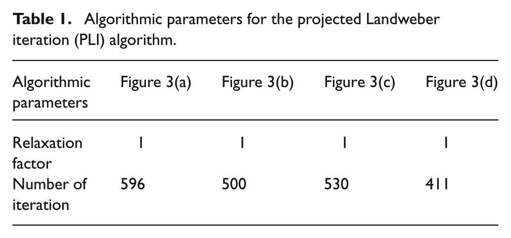
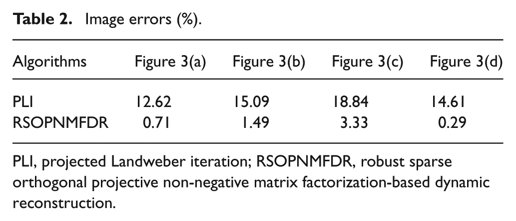
Image errors (%).
PLI, projected Landweber iteration; RSOPNMFDR, robust sparse orthogonal projective non-negative matrix factorization-based dynamic reconstruction.
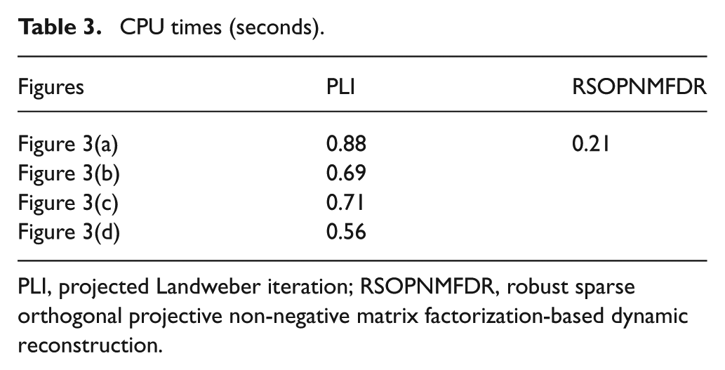
CPU times (seconds).
PLI, projected Landweber iteration; RSOPNMFDR, robust sparse orthogonal projective non-negative matrix factorization-based dynamic reconstruction.
Figure 4 shows the images reconstructed by the PLI algorithm. Owing to the fact that only gradient information of the objective functional is used in implementing image reconstruction, the numerical implementation of the PLI algorithm is easy and the computational complexity is low. In the past years, the PLI algorithm had found numerous applications in different fields of the inverse problems, including ECT image reconstruction. Like other static reconstruction algorithms, unfortunately, the PLI algorithm merely utilizes the ECT measurement information, and fails to consider the dynamic evolution information and the temporal correlations of a dynamic object, which is not optimal for the dynamic reconstruction tasks. In fact, it can be found from Figure 4 that in the case of the dynamic reconstruction, the quality of the images reconstructed by the PLI method is far from perfect, the distortions are serious, and the detailed edge information of the reconstructed images is blurred. It can be observed form Table 2 that the image errors of the PLI algorithm for dynamic reconstruction objects, Figures 3(a)–(d), are 12.62%, 15.09%, 18.84% and 14.61%, which are higher than that of the RSOPNMFDR algorithm.
Figure 5 is the images reconstructed by the RSOPNMFDR algorithm. Numerical simulation results indicate that the RSOPNMFDR algorithm can ensure the numerical stability of an inversion solution owing to the fact that the Tikhonov regularization technique is employed, and the computational cost is low due to the dimensionality reduction of the original unknown variables. In particular, the RSOPNMFDR algorithm simultaneously utilizes the ECT measurement information and the dynamic evolution information of a dynamic object, and thus the quantity of information is increased, which facilitates the improvement of the reconstruction quality. It can be seen from Figure 5 that the quality of the images reconstructed by the RSOPNMFDR algorithm is improved compared with the PLI method. Furthermore, it can be seen from Table 2 that the image errors of the RSOPNMFDR algorithm for dynamic reconstruction objects, Figures 3(a)–(d), are 0.71%, 1.49%, 3.33% and 0.29%, which are lower than that of the PLI algorithm.
The image errors for the PLI method and the RSOPNMFDR algorithm are listed in Table 2. As can be expected, the reconstruction quality of the RSOPNMFDR algorithm is superior to the PLI method. Furthermore, it can be observed from Table 2 that for the cases simulated in this section, the RSOPNMFDR algorithm gives the smallest image errors, which indicates that the RSOPNMFDR algorithm is a promising candidate for solving ECT image reconstruction problems.
ECT measurement objects are often in a time-vary process, and achieving fast reconstruction is crucial for real applications. Based on the multiple measurement vectors model and the dimensionality reduction of the unknown variables, in the RSOPNMFDR algorithm the images are indirectly reconstructed by solving the corresponding low-dimensional coefficient vector in a batching pattern, which differs from existing reconstruction algorithms. Owing to the dimensionality reduction of the original unknown variables, especially, the reconstruction speed is improved and the CPU times are reduced. In fact, it can be found from Table 3 that the CPU times of the RSOPNMFDR algorithm for reconstructing Figures 3(a)–(d) are about 0.21 s, which is significantly fewer than that of the PLI method, 2.84 s. This advantage is highly appropriate for real applications.
Case 3
The ECT image reconstruction process is an ill-posed problem, and small perturbations in input data may lead to a large fluctuation of an inversion solution, which may make the final solution meaningless. In practice, measurement noises are ubiquitous and complicated. A successful algorithm should be able to deal with such problem. In this section, the noise-contaminated capacitance data is used to evaluate the robustness of the RSOPNMFDR algorithm, and the definition of the noise level can be specified as:
where
Algorithmic parameters for the RSOPNMFDR algorithm are the same as above. Figures 6–8 illustrate the images reconstructed by the RSOPNMFDR algorithm under the noise levels of 5%, 16% and 30%, respectively. The image errors are listed in Table 4.
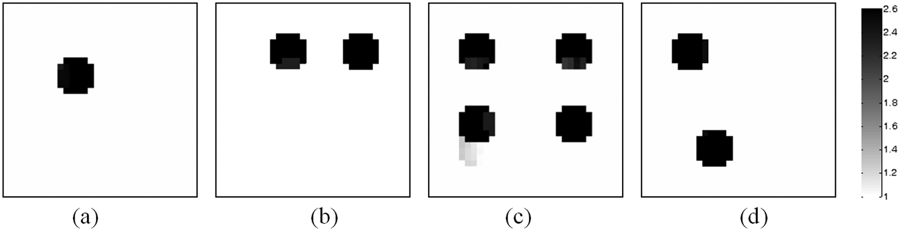
Reconstructed images by the robust sparse orthogonal projective non-negative matrix factorization-based dynamic reconstruction (RSOPNMFDR) algorithm under the noise level of 5%.
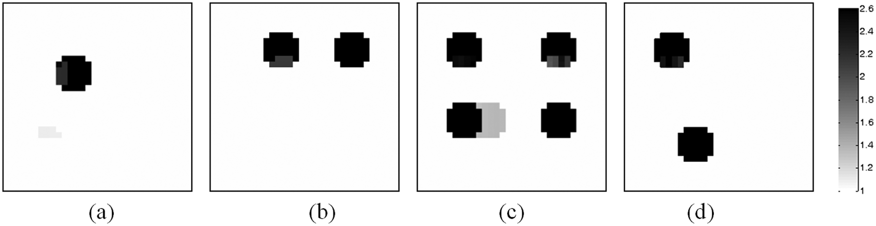
Reconstructed images by the robust sparse orthogonal projective non-negative matrix factorization-based dynamic reconstruction (RSOPNMFDR) algorithm under the noise level of 16%.
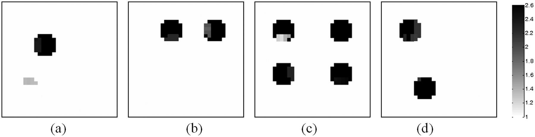
Reconstructed images by the robust sparse orthogonal projective non-negative matrix factorization-based dynamic reconstruction (RSOPNMFDR) algorithm under the noise level of 30%.
Image errors (%).
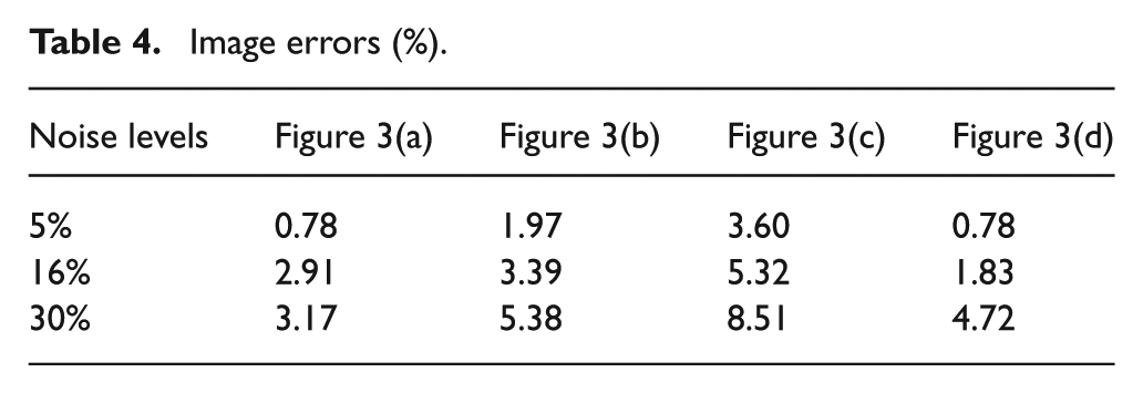
Figures 6 –8 show the images reconstructed by the RSOPNMFDR algorithm under the noise levels of 5%, 16% and 30%, respectively. Owing to the fact that the M-estimation technique and the Tikhonov regularization method are introduced to the proposed objective functional, as can be expected, the RSOPNMFDR algorithm shows satisfactory robustness, and the reconstructed images under different noise levels are in a good agreement with the original dynamic objects. In particular, it can be observed from Table 4 that when the noise level is 30%, the image errors for the original reconstruction objects, Figures 3(a)–(d), are 3.17%, 5.38%, 8.51% and 4.72%, respectively. Additionally, owing to the fact that the dimensionality of the unknown variables in the RSOPNMFDR algorithm, the ill-posed property may be therefore alleviated, finally the sensitivity of the inversion solution to measurement noises is decreased.
Case 4
It is worth emphasizing that in real applications the sensitivity matrix is often inaccurate derived from physically implementing an imperfect ECT sensor and the approximation solution of the sensitivity matrix, and thus a successful algorithm should be able to deal with such inaccuracy. In this section, the influence of the inaccuracy of the sensitivity matrix on the reconstruction quality is evaluated, and the inaccuracy of the sensitivity matrix is defined as:
where
Algorithmic parameters for the RSOPNMFDR algorithm are the same as before. Figures 9 and 10 illustrate the images reconstructed by the RSOPNMFDR algorithm when the standard deviations of the sensitivity matrix are 0.002 and 0.004, respectively. The image errors are presented in Table 5.
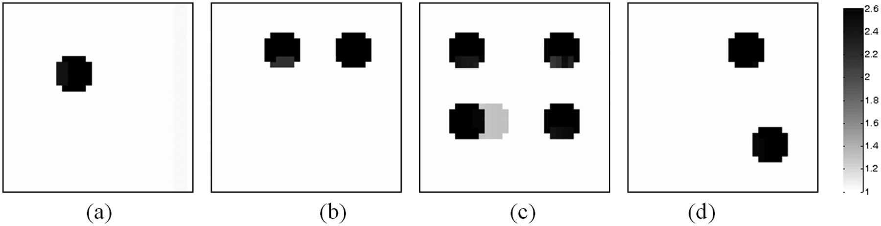
Reconstructed images when the standard deviation of the sensitivity matrix is 0.002.
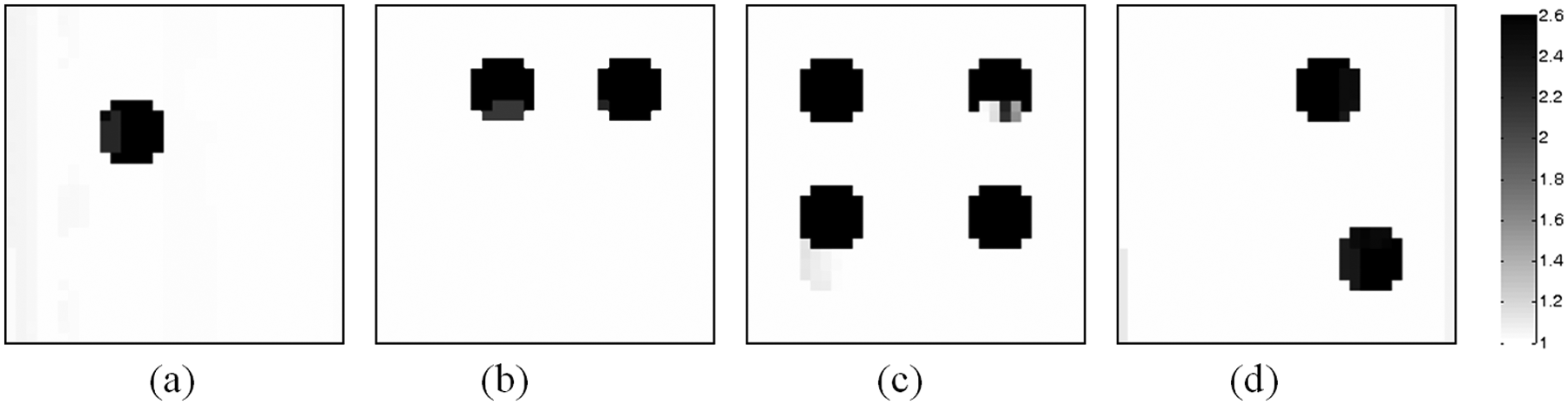
Reconstructed images when the standard deviation of the sensitivity matrix is 0.004.
Image errors (%).
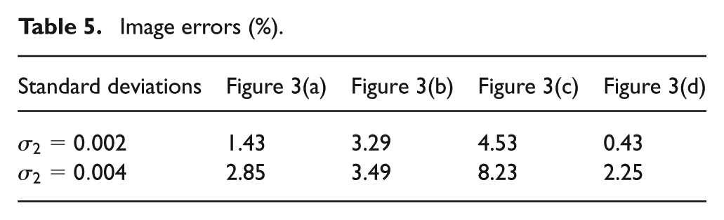
When the standard deviations of the sensitivity matrix are 0.002 and 0.004, the images reconstructed by the RSOPNMFDR algorithm are shown in Figures 9 and 10, respectively. It can be observed from Figures 9 and 10 that owing to the fact that the inaccurate property of the sensitivity matrix is considered in the proposed objective functional, the quality of the images reconstructed by the RSOPNMFDR algorithm under the conditions of the inaccuracy of the sensitivity matrix is satisfactory. Particularly, it can be seen from Table 5 that when the standard deviation of the sensitivity matrix is 0.004, the image errors for the original dynamic reconstruction objects, Figures 3(a)–(d), are 2.85%, 3.49%, 8.23% and 2.25%, which indicates that the RSOPNMFDR algorithm is robust to the inaccuracy of the sensitivity matrix.
Case 5
In order to further evaluate the robustness of the RSOPNMFDR algorithm, in this section the influences of the inaccuracies of the sensitivity matrix and the measurement data on the reconstruction quality are studied. In this case, algorithmic parameters for the RSOPNMFDR algorithm are the same as before. Figures 11 and 12 illustrate the images reconstructed by the RSOPNMFDR algorithm when the inaccurate properties on the sensitivity matrix and the measurement data, and the image errors are presented in Table 6.
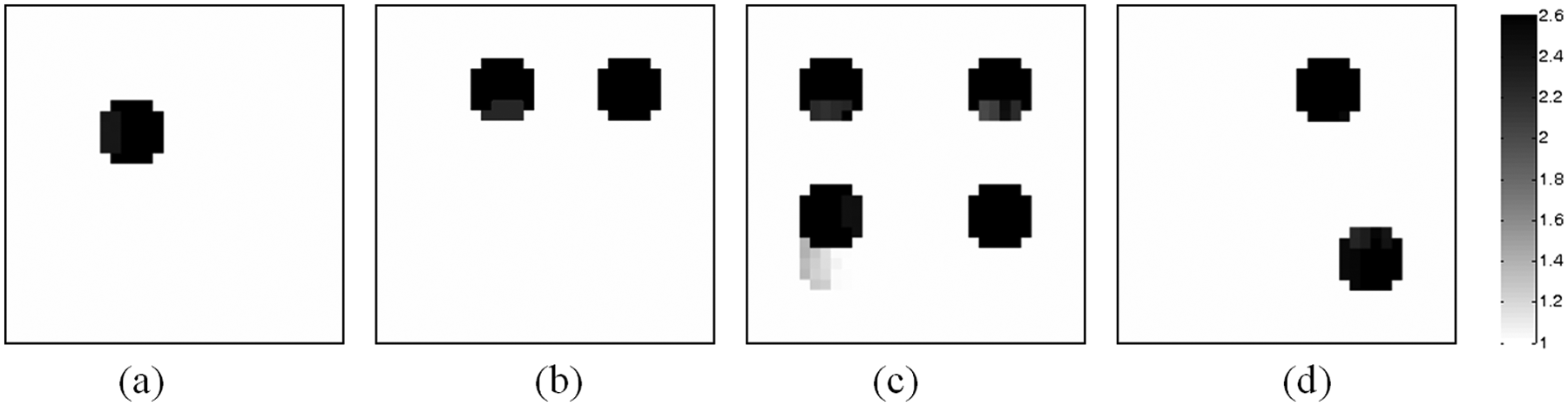
Reconstructed images when the standard deviation of the sensitivity matrix and the noise level of the capacitance data are 0.001 and 5%.
Reconstructed images when the standard deviation of the sensitivity matrix and the noise level of the capacitance data are 0.003 and 10%.
Image errors (%).
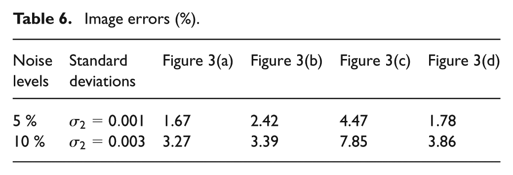
Figures 11 and 12 present the images reconstructed by the RSOPNMFDR algorithm when the inaccurate properties on the sensitivity matrix and the measurement data are simultaneously considered. It can be observed from Figures 11 and 12 that owing to the fact that the inaccurate properties on the sensitivity matrix, the measurement data and the reconstruction model are considered in the proposed objective functional and the ill-posed nature is illustrated via the dimensionality-reduction of the unknown variables, the quality of the images reconstructed by the RSOPNMFDR algorithm under the conditions of the inaccuracies of the sensitivity matrix and the measurement data is satisfactory. In particular, it can be seen from Table 6 that when the standard deviation of the sensitivity matrix is 0.003 and the noise level of the capacitance data is 10%, the image errors for the original dynamic reconstruction objects, Figures 3(a)–(d), are 3.27%, 3.39%, 7.85% and 3.86%, which confirms that the RSOPNMFDR algorithm is robust to the inaccuracies of the sensitivity matrix and the measurement data.
Case 6
In this section the noise-contaminated capacitance data is used to further evaluate the robustness of the RSOPNMFDR algorithm. Subfigures (a), (b) and (c) in Figure 13 stand for the different permittivity distributions at time instants
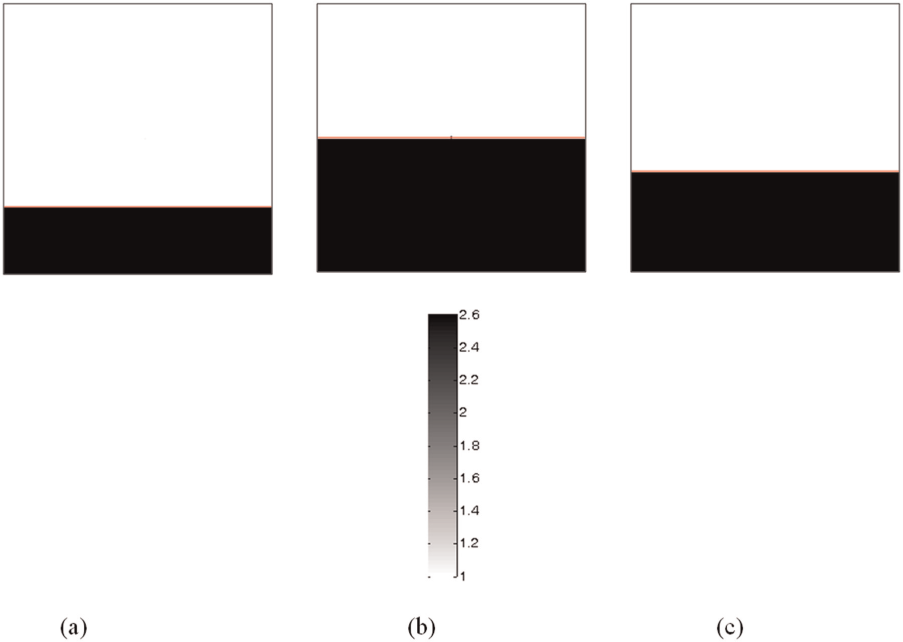
Reconstruction objects.
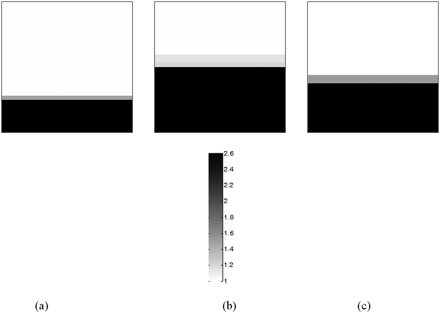
Reconstructed images by the robust sparse orthogonal projective non-negative matrix factorization-based dynamic reconstruction (RSOPNMFDR) algorithm under the noise level of 3%.
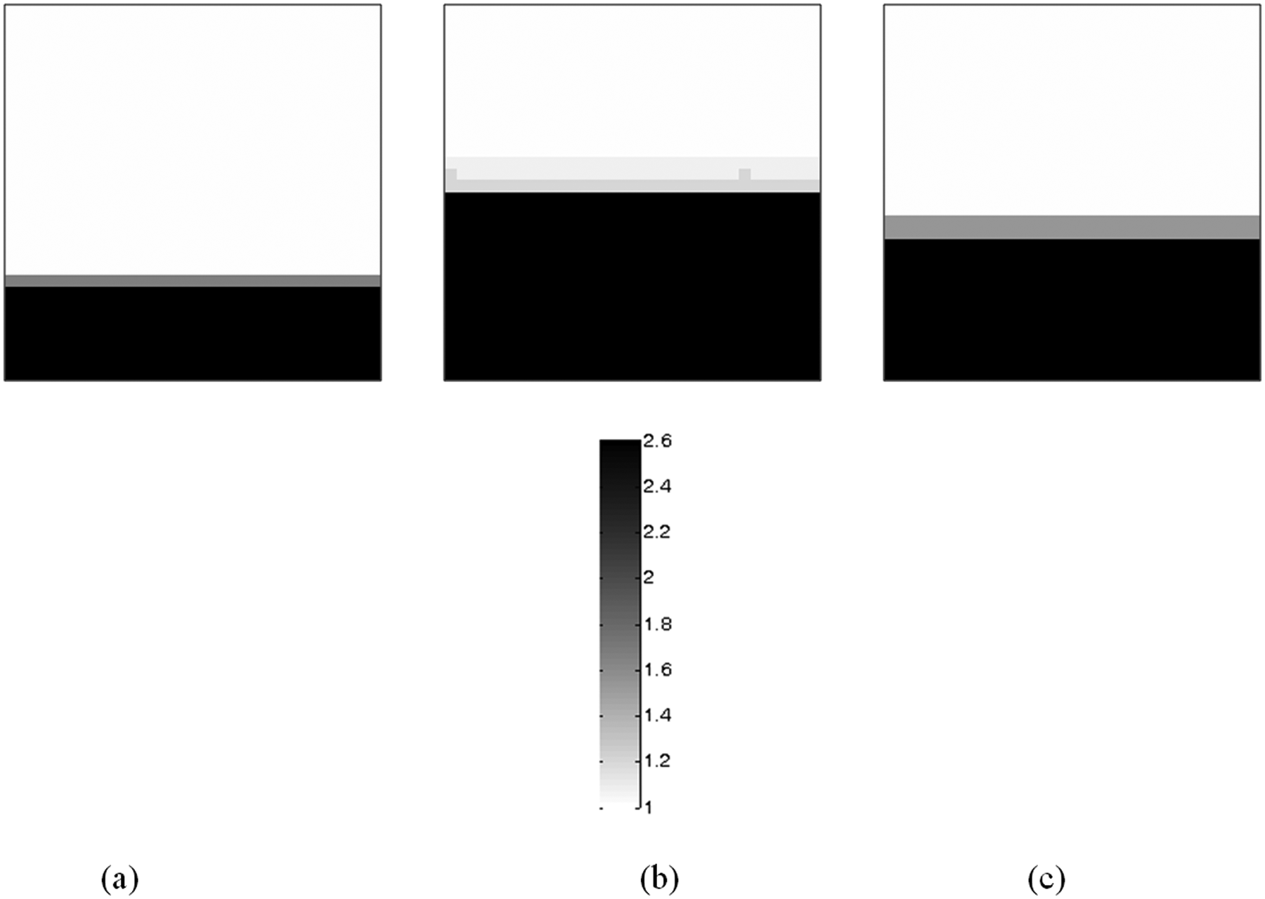
Reconstructed images by the robust sparse orthogonal projective non-negative matrix factorization-based dynamic reconstruction (RSOPNMFDR) algorithm under the noise level of 8%.
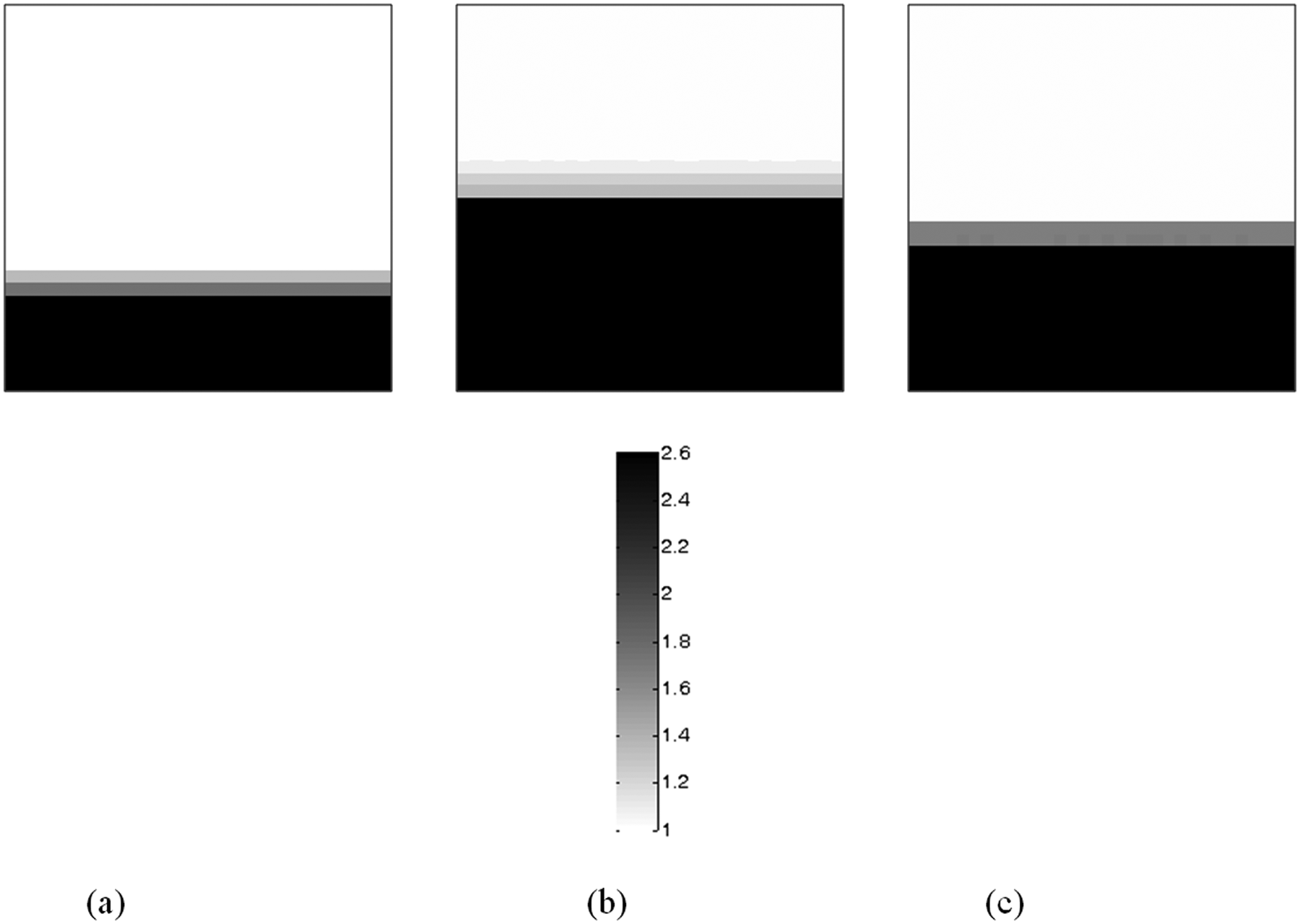
Reconstructed images by the robust sparse orthogonal projective non-negative matrix factorization-based dynamic reconstruction (RSOPNMFDR) algorithm under the noise level of 15%.
Image errors (%).
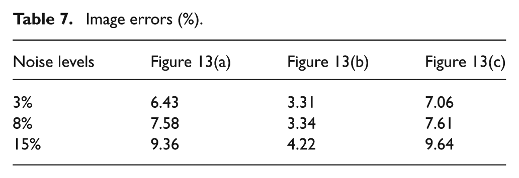
Figures 14 –16 show the images reconstructed by the RSOPNMFDR algorithm under the noise levels of 3%, 8% and 15%, respectively. Owing to the fact that the M-estimation technique and the Tikhonov regularization method are introduced to the proposed objective functional, as can be expected, the RSOPNMFDR algorithm shows satisfactory robustness, and the reconstructed images under different noise levels are in a good agreement with the original dynamic objects. It can be observed from Table 7 that the RSOPNMFDR algorithm is robust to the inaccuracies of the measurement data. However, it can be found from Table 7 that the image errors increase with the rising noise levels, which indicates that the measurement noises needs to be carefully tackled in real applications, and this issue should be further investigated in the future.
Case 7
In this section, the effect of the number of the basis vector on the reconstruction quality is numerically evaluated. Figure 17 shows the image errors of the RSOPNMFDR algorithm for original dynamic reconstruction objects under different numbers of the basis vectors.
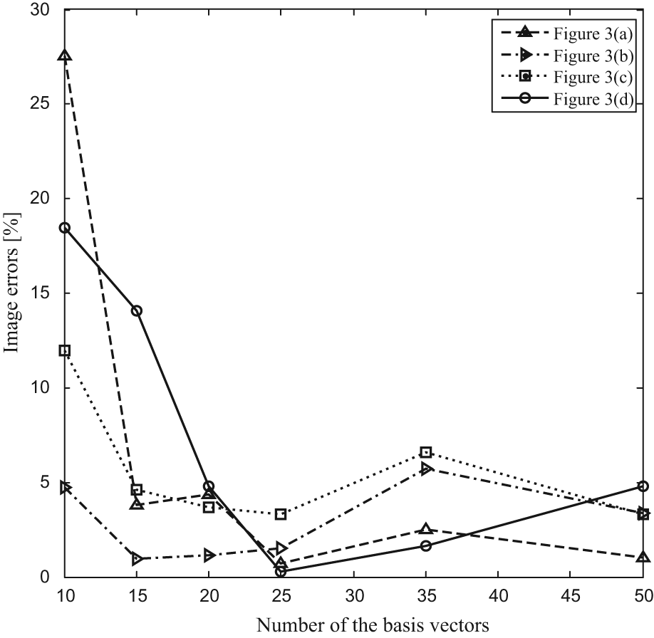
Image errors under different numbers of the basis vectors.
Following the discussions presented in previous sections, it can be seen that differing from existing reconstruction methods, in the RSOPNMFDR algorithm the images are indirectly reconstructed by solving a low dimensional coefficient vector. It can be found from Figure 17 that for the dynamic reconstruction cases presented in this paper, the number of the basis vectors will affect the reconstruction quality, which indicates that the snapshots that are used to solve the basis vectors should be cautiously determined. In fact, previous studies indicate that the basis vectors from a poor set of snapshots may impede the improvement of the reconstruction quality.
The simulation results presented in previous sections indicate that the RSOPNMFDR algorithm is a promising candidate for imaging the dynamic reconstruction objects. However, it is worth emphasizing that this paper presents a general framework for solving inverse problems in dynamic image reconstruction tasks, which may be useful for the image reconstruction problems in other related fields.
Conclusions
ECT image reconstruction process is an ill-posed problem, in which the accuracy and speed of image reconstruction algorithms play a crucial role in real applications. In this paper, a multiple measurement vector-based dimensionality reduction dynamic reconstruction model that utilizes the ECT measurement information and the dynamic evolution information of a dynamic object is proposed. A RSOPNMF method is proposed for extracting the basis vectors from a set of snapshots, and the SBI method is used to solve the RSOPNMF model. The original unknown variables are projected onto the subspaces spanned by a set of the basis vectors extracted by the RSOPNMF method from a set of snapshots to obtain a low-dimensional model where the images are indirectly reconstructed by solving the corresponding coefficients, and thus the dimensionality of the unknown variables is reduced and the reconstruction speed is improved. Based on the multiple measurement vectors and the dimensionality reduction model, an objective functional that incorporates the ECT measurement information, the dynamic evolution information of a dynamic object, the spatial constraint and the temporal constraint is proposed, in which the unknown variables are solved in a batching pattern. An iterative scheme that integrates the beneficial advantages of the SBI method and the FBS algorithm is developed for solving the proposed objective functional. Numerical simulation results indicate that the proposed algorithm is advantageous on the improvement of the reconstruction quality and the reconstruction speed. As a result, a promising algorithm is provided for solving ECT inverse problems.
Applications indicate that different algorithm may obtain different numerical results when different reconstruction tasks are implemented, and the choice of a specific reconstruction algorithm depends mainly on the measurement requirements and the understanding of a reconstruction object. Our work provides a candidate method for solving ECT image reconstruction problems, which needs to be further validated by more cases and improved in the future.
Footnotes
Funding
The authors wish to thank the National Natural Science Foundation of China (grant number 51206048) and the Fundamental Research Funds for the Central Universities (grant number 13MS11) for supporting this research.