






Abstract
This paper is associated with the problem of robust stability of discrete-time systems with time-varying delays and finite wordlength nonlinearities. The main contribution of the paper is two-fold. First, this paper presents a new Lyapunov function based on the idea of partitioning the delay interval into subintervals. The approach may be considered as an advancement over the several existing approaches where only the lower delay bound is partitioned. The second is that reciprocally convex inequality (RCI) and Wirtinger-based inequality (WBI) are used to estimate the sum terms involved in the forward difference of Lyapunov function. The intermediate delay is also included in the Lyapunov function to deal with the delay information more effectively. Finally, several examples are provided to illustrate the less conservatism of the proposed approach as compared to several existing results.
Keywords
Introduction
Over the past few decades, many researchers have paid attention to the stability analysis and design of the discrete-time systems with time delay due to their extensive applications in various fields such as networked control system, neural networks, microgrid system and so on (Mary and Rangarajan, 2016; Naghshtabrizi et al., 2010; Peng et al., 2011; Yu et al., 2013). During the implementation of discrete-time systems on the finite wordlength digital processor, the quantization (roundoff, magnitude truncation and value truncation) and overflow (saturation, zeroing, 2’s complement and triangular) nonlinearities are frequently introduced. These nonlinearities may cause the oscillations typically known as the limit cycles and push the system towards instability (Butterweck et al., 1988; Chang, 1981; Erickson and Michel, 1985). It is essential to find the range of the system parameters for limit cycle-free implementation of the system. Several criteria for the stability of discrete-time systems with quantization nonlinearities have been reported in Bose (1994), Chang (1981) and Lepschy et al. (1988) by ignoring the overflow effects, whereas others (Ahn and Kar, 2015a, 2015b; Chen, 2009; Kandanvli and Kar, 2008, 2009a; Kar, 2007; Kokil et al., 2020; Singh, 2010) have studied the overflow effects in discrete-time systems without considering the quantization effects. The effects of the combination of overflow and quantization are investigated in Kandanvli and Kar (2009b, 2011), Mahmoud (2013), Tadepalli et al. (2015, 2018) and Tadepalli and Kandanvli (2016, 2017).
Apart from above instability sources, the existence of time delays and parameter uncertainties in the discrete-time systems also lead to system instability. Parameter uncertainties occur in the system due to the variation of system parameters and modelling errors. Time delays are inevitable which are encountered if there is transmission of data from one part of the system to another. These delays deeply manipulate the stability of the system and offer deprived performance of the system (Feng et al., 2015; Kwon et al., 2013; Lee and Tsai, 2013; Li et al., 2018; Liu and Zhang, 2012; Mary and Rangarajan, 2016; Meng et al., 2010; Naghshtabrizi et al., 2010; Nam et al., 2015; Seuret et al., 2015; Shao and Han, 2011; Xu et al., 2014; Xue et al., 2016; Yu et al., 2013). Several researchers have explored the stability of uncertain discrete-time systems with time delay (see, Chen et al., 2004; Gao and Chen, 2007; Hua et al., 2014; Huang and Feng, 2010; Xu et al., 2001).
During the last decade, several papers dealing with the construction of suitable Lyapunov functions for analyzing the stability of discrete systems with time-varying delays have appeared (Feng et al., 2015; Gao and Chen, 2007; Kwon et al., 2013; Meng et al., 2010; Nam et al., 2015; Xu et al., 2014; Zhang et al., 2008). During the estimation of forward difference of Lyapunov functions, several techniques (e.g., free weighting matrix (FWM)-based method, inequality-based method etc.) are employed to handle the sum terms. FWM-based method uses the bounding inequalities for cross product between two vectors to reduce the conservatism of the stability conditions. However, this method introduces free weighting matrices, and hence, computationally demanding. In inequality-based method, the sum term is estimated by utilizing the well-known inequalities. Examples of inequality-based methods reported in the literature are reciprocally convex inequality (RCI) method (Liu and Zhang, 2012; Park et al., 2011), Jensen-based inequality (JBI) method (Huang and Feng, 2010; Liu and Zhang, 2012; Tadepalli and Kandanvli, 2016, 2017; Tadepalli et al., 2015; Xu et al., 2014) and Wirtinger-based inequality (WBI) method (Chen et al., 2016; Nam et al., 2015; Seuret et al., 2015; Tadepalli et al., 2018). The RCI is bounded inequality lemma for a linear combination of positive functions where the coefficients are inverses of convex parameters. This approach is usually less conservative than convex combination approach and also requires less decision variables. JBI approach approximates the difference of delay bounds due to the inversely weighted nature of coefficients to improve stability of the system. Criteria derived by WBI method generally provide less conservatism results than those obtained via JBI method (Seuret et al., 2015; Tadepalli et al., 2018). However, all these methods still convey the conservatism to some extent.
From the designer’s point of view, it is important to know the admissible maximum delay bound such that the system with delay less than this bound remains stable. One major concern to find the maximum admissible upper bound is to reduce the conservatism of criteria. In Kandanvli and Kar (2008, 2009a), delay-independent conditions are developed for the stability of discrete systems with constant delays, overflow nonlinearities and uncertainties. A delay-dependent criterion has been derived in Chen (2009) for systems with saturation nonlinearities and time-varying delays. By employing FWM method, Kandanvli and Kar (2011) established a delay-dependent stability criterion for systems with time-varying delays and composite nonlinearities. The stability criteria in Tadepalli and Kandanvli (2016) utilize the concepts of JBI and delay partitioning approach. The criteria in Tadepalli et al. (2018) are derived by adopting the WBI approach which provide less stringent results as compared to Tadepalli and Kandanvli (2016).
To further reduce the conservatism, delay partitioning technique may be adopted which can provide better stability results for the system. This technique is firstly used in Meng et al. (2010) to tackle with stability of the system. The approaches in Meng et al. (2010) and Tadepalli and Kandanvli (2016) are based on partitioning the lower bound of the interval-like time-varying delay only. It makes such approaches less effective if the lower delay bound is 0 or 1 and also the delay information is not exploited adequately. Thus, the derivation of less conservative stability criteria is still an important and challenging research problem.
In order to overcome the limitations in Meng et al. (2010) and Tadepalli and Kandanvli (2016) and utilize the delay information more effectively, in this paper, we have partitioned the delay interval into
The aim of this paper is to establish delay-dependent stability criteria for discrete-time systems with parameter uncertainties, delays, quantization and overflow nonlinearities. The contribution of the paper is as follows. Firstly, the system is studied by partitioning the delay interval into
The paper is planned as follows. The next section gives the description of the system in state variable form. Based on delay partitioning approach, new stability criteria for uncertain discrete-time systems involving time-varying delays and finite wordlength nonlinearities are proposed in ‘Main Results’ section. A global asymptotic stability result for the considered system in absence of uncertainties and nonlinearities is also presented in this section. The advantages of the proposed results are illustrated with the help of numerical examples along with simulation results in ‘Examples’ section. The final section concludes the paper.
System description
This section presents the description of the system under consideration and the problem statement. Some useful lemmas needed for deriving our main results, are also provided.
Consider a class of discrete-time systems influenced by a combination of quantization and overflow nonlinearities, parameter uncertainties and time-varying delays. In particular, the system under consideration is given by
where
The d(r) is a time-varying delay such that
where
Here, the intermediate delay
where the notation
Similarly, for the case where
The uncertainties are included as
where
A class of discrete-time delayed systems consisting of parameter uncertainties, quantization and overflow nonlinearities can be described by the equations (1), (2) and (6). These systems cover digital control systems with quantization/overflow (Mahmoud, 2013), metal cutting process, material rolling process, wireless sensor networks (Chakrabarty et al., 2002) and so forth. Distinctive examples where the time delays, represented by (2), can occur in various communication networks during the transmission of signals like networked control system (NCS), microgrid system (MGS) and so on (Mary and Rangarajan, 2016; Peng et al., 2011). In the analysis of NCS, network induced delay and packet dropout are most important factors. MGS controller transmits the information in open communication networks that introduces some communication delay in the system.
The aim of this paper is to analyse the stability of the discrete-time system (1) and to establish less conservative stability condition by adopting an effective delay-partitioning approach.
The following lemmas are helpful for establishing the main results of the paper.
then
where
then
where
Main results
This section presents the main results of the paper.
For the given system (1) which is operating in presence of quantization and overflow,
where
The delay partitioning is one of the very promising methods in reducing the conservativeness of the derived stability criteria. To present our approach in a lucid manner, we proceed with
Pertaining to
where
The proof of Theorem 1 is given in Appendix I.
with
From Remark 1 of Seuret et al. (2015) and Remark 6 of Tadepalli et al. (2018), it may be noted that (15) is less restrictive than that obtained via JBI. (iii) Unlike estimating the simple difference between upper and lower delay bounds to use a convex combination approach, the RCI approach treats with the inversely weighted convex combination of quadratic sum terms (Feng et al., 2015).
Pertaining to the situation where the delay interval is partitioned into three parts (i.e.,
where
As a direct consequence of Theorem 1, we have the following corollary for the system (1) and (2) in absence of parameter uncertainties and finite wordlength nonlinearities.
Then the system represented by (18) and (2) is globally asymptotically stable for given positive integers
where
The proof of Corollary 1 is given in Appendix III.
Examples
This section provides the numerical examples for illustrating the utility of the proposed criteria.
Let the nonlinearities in the system are confined to
The maximum allowed
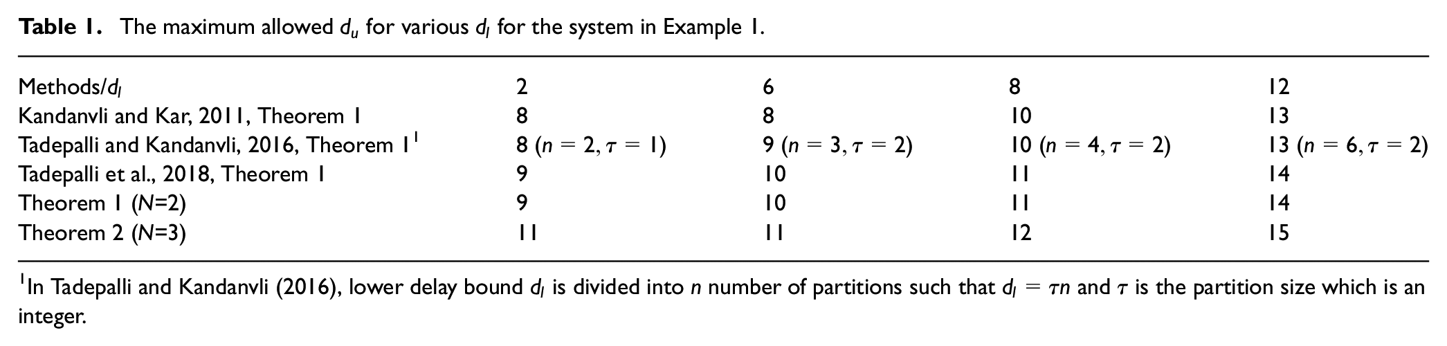
1In Tadepalli and Kandanvli (2016), lower delay bound
From Table 1, it is clear that Theorem 2 yields fewer conservative results than Theorem 1 in Kandanvli and Kar (2011), Theorem 1 in Tadepalli and Kandanvli (2016) and Theorem 1 in Tadepalli et al. (2018) for the present example. Theorem 1 provides the same upper bound
Figure 1 shows a plot of state trajectories of the system in Example 1 with an arbitrary initial condition,
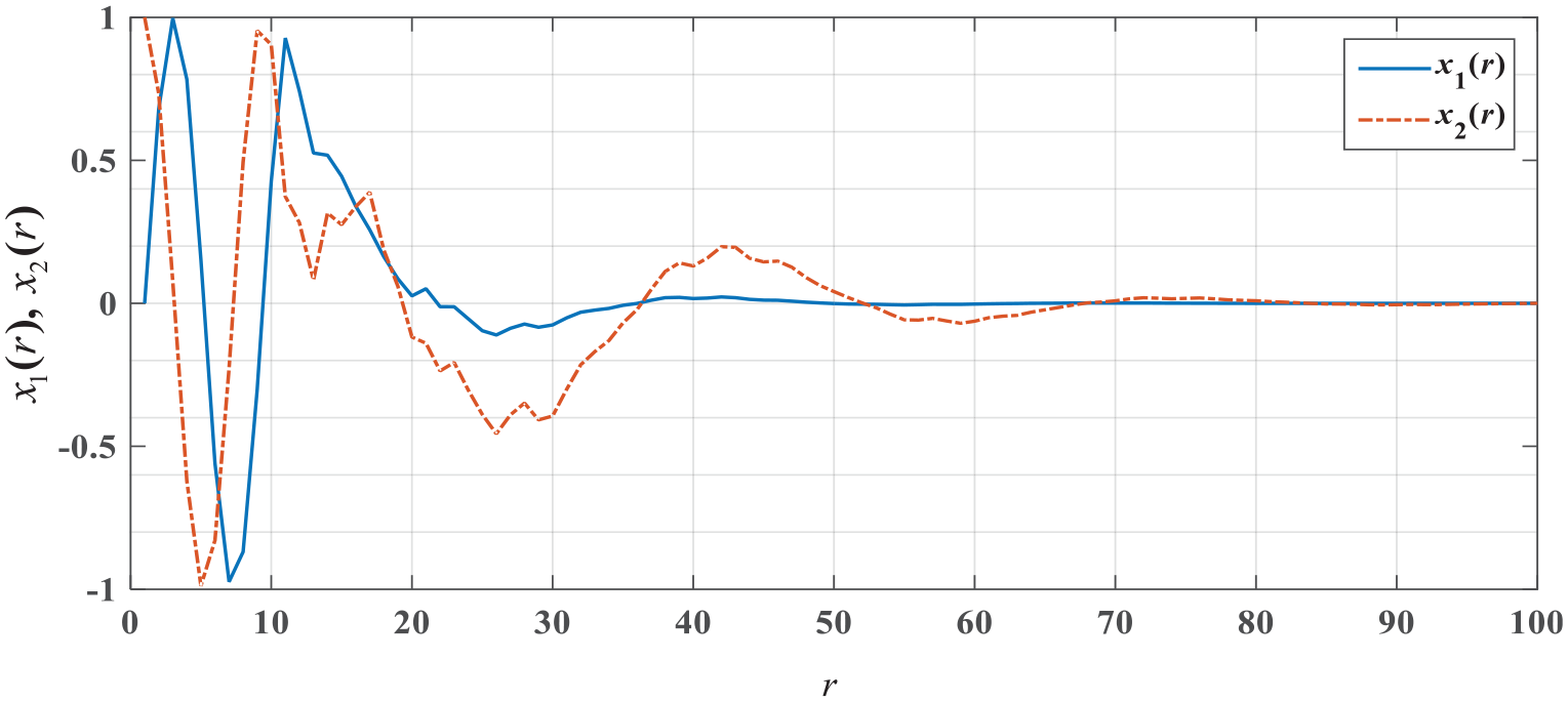
State trajectories of the system for Example 1.
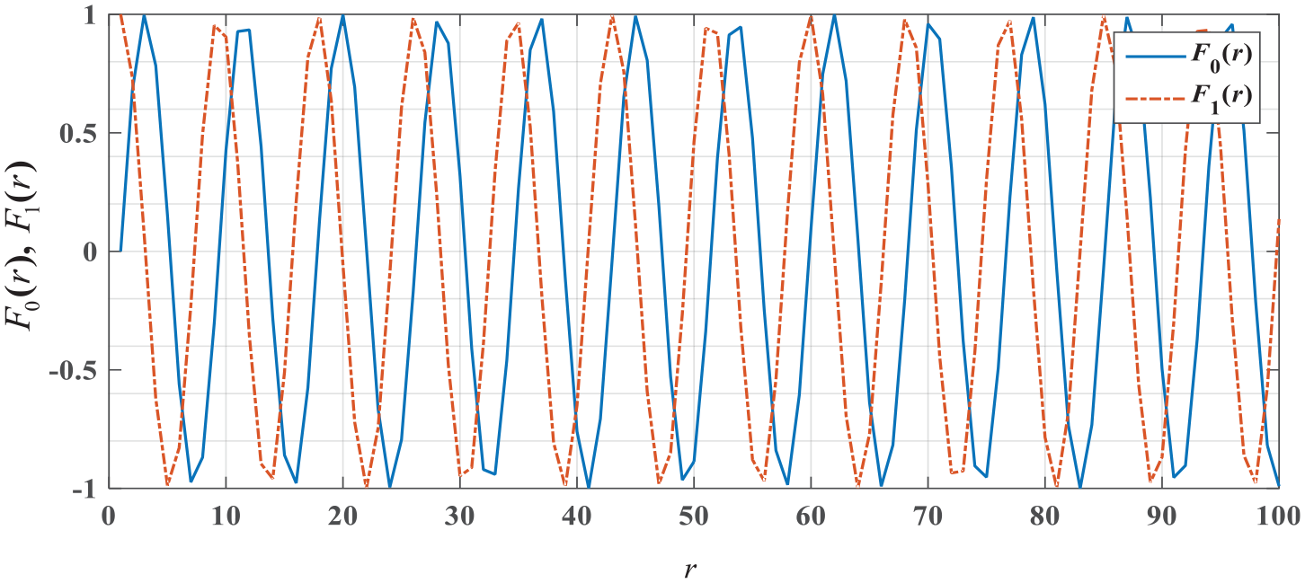
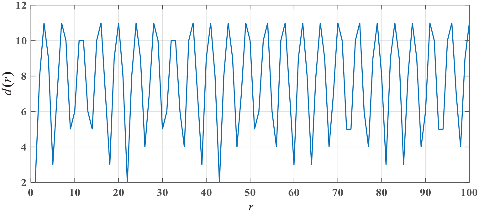
Time-varying delay d(r) used in the simulation for Example 1.
The admissible maximum delay bounds for given lower delay bounds obtained via various criteria for the global asymptotic stability of present system are listed in Table 2. From Table 2, one can infer that the proposed criteria (Theorems 1 and 2) provide reduced conservatism than the existing ones (Kandanvli and Kar, 2011; Tadepalli and Kandanvli, 2016; Tadepalli et al., 2018) for this example.
The maximum allowed

The state trajectories for the present system with an arbitrary initial condition,
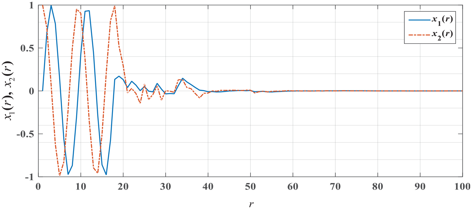
State trajectories of the system for Example 2.
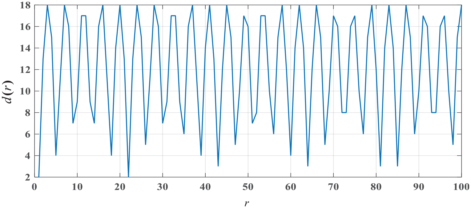
Time-varying delay d(r) used in the simulation for Example 2.
The global asymptotic stability of this example was investigated in Chen et al. (2017), Feng et al. (2015) and Liu and Zhang (2012). For given
The maximum allowed

As the number of subintervals ‘N’ becomes larger (≥2), the conservatism of the delay-dependent stability results is reduced while the computational burden increases. This is obvious from Theorems 1 and 2 as the number of decision variables D is directly related to the number of subintervals N. In other words, a larger N implies that the feasibility solution can be explored in a larger set which is confirmed by the results obtained in Examples 1 and 2 (see Tables 1 and 2 also). On the other hand, the increase of number of decision variables results in heavier computational burden. The total number of decision variables for the case N=2 (Theorem 1) is
Pertaining to the system (1), (2), (6) and (12), in the general case, the relation between the total number of decision variables D and the number of subintervals N in the approach adopted in this paper is obtained as
Conclusions
This paper has discussed the problem of delay-dependent stability of uncertain discrete-time systems with time-varying delays and under the influence of quantization and overflow nonlinearities. Two LMI-based delay-dependent criteria (Theorems 1 and 2) have been proposed. Suitable Lyapunov functions are constructed that involve intermediate delays that utilize the delay information more effectively in the proposed criteria. To deal with the sum terms, WBI approach together with RCI approach has been utilized. As illustrated in Examples 1 and 2, Theorem 2 can provide less conservative results as compared with Theorem 1. The presented approach yields improved stability results as compared to previous methods (Kandanvli and Kar, 2011; Tadepalli and Kandanvli, 2016; Tadepalli et al., 2018). Though the stability results have been established in this paper for N=2 and 3, the stability criterion corresponding to a general N can easily be worked out. A global asymptotic stability result (Corollary 1) for the underlying system in absence of uncertainties and nonlinearities is also brought out.
Though the stability criteria proposed in this paper deal with systems with single time-varying delay, the approach can be easily extended to establish the global asymptotic stability criterion for systems with multiple time-varying delays. The problem of obtaining improved stability conditions by combining the presented approach and the ideas of nonuniform delay partitioning (Feng et al., 2015) requires further investigation. The possible extension of the presented approach to develop delay-dependent stability criteria for 2-D uncertain systems (Peng et al., 2018; Tadepalli et al., 2015) is an interesting problem for future investigation. The possible deployment of the presented ideas for developing delay-dependent stability criteria for 1-D and 2-D uncertain discrete time-varying delayed systems with finite wordlength nonlinearities and external interferences (Ahn and Kar, 2015a, 2015b; Kokil et al., 2020) appears to be a realistic and challenging problem for further study.
Footnotes
Appendix I
Proof of Theorem 1: Consider a Lyapunov function as
with
where
The forward difference of Lyapunov function (A.1) along the trajectories of the system (1) is
where
Using Lemma 1, it can be shown that
Now, consider the two possible cases:
In this case, the terms in
where
By utilizing Lemmas 1 and 2, the sum terms in
The validity of (A.7) lies in the fact (see Lemma 2) that if there exists a matrix
Next, using (A.4)–(A.8), one obtains
where
Note that, in light of (12), the quantity ‘a’ (see (A.10)) is non-negative (Kandanvli and Kar, 2009b; Kar and Singh, 2001; Tadepalli et al., 2018). Therefore, the condition
By Schur’s complement, the condition
where
In view of (6a), (A.12) can be rearranged as
where
By employing Lemma 3, (A.13) is equivalent to
Using Schur’s complement, (A.17) can also be written as
where
Following similar mathematical treatment as shown in equations (A.13)–(A.18), it is easy to show that (A.18) is equivalent to the condition
In this case, by adopting the similar procedure as considered in Case I for
where
and
Note that the existence of the matrix
It is obvious that
Appendix II
One can easily arrive at Theorem 2 by employing the Lyapunov function
where
and following the steps shown in the proof of Theorem 1.
Appendix III
Acknowledgements
The authors wish to thank the Editor, the Associate Editor and the anonymous reviewers for their constructive comments and suggestions.
Declaration of conflicting interests
The author(s) declared no potential conflicts of interest with respect to the research, authorship, and/or publication of this article.
Funding
The author(s) received no financial support for the research, authorship, and/or publication of this article.
